Note
Go to the end to download the full example code.
PDHG and LM-SPHG to optimize the Poisson logL and total variation
This example demonstrates the use of the primal dual hybrid gradient (PDHG) algorithm, the listmode stochastic PDHG (LM-SPDHG) to minimize the negative Poisson log-likelihood function combined with a total variation regularizer:
subject to
using the linear forward model
Tip
parallelproj is python array API compatible meaning it supports different
array backends (e.g. numpy, cupy, torch, …) and devices (CPU or GPU).
Choose your preferred array API xp and device dev below.
Warning
Running this example using GPU arrays (e.g. using cupy as array backend) is highly recommended due to “longer” execution times with CPU arrays
36 from __future__ import annotations
37
38 import array_api_compat.cupy as xp
39
40 # import array_api_compat.numpy as xp
41 # import array_api_compat.torch as xp
42
43 import parallelproj
44 from array_api_compat import to_device
45 import array_api_compat.numpy as np
46 import matplotlib.pyplot as plt
47
48 # choose a device (CPU or CUDA GPU)
49 if "numpy" in xp.__name__:
50     # using numpy, device must be cpu
51     dev = "cpu"
52 elif "cupy" in xp.__name__:
53     # using cupy, only cuda devices are possible
54     dev = xp.cuda.Device(0)
55 elif "torch" in xp.__name__:
56     # using torch valid choices are 'cpu' or 'cuda'
57     if parallelproj.cuda_present:
58         dev = "cuda"
59     else:
60         dev = "cpu"
Input Parameters
65 # image scale (can be used to simulated more or less counts)
66 img_scale = 0.1
67 # number of MLEM iterations to init. PDHG and LM-SPDHG
68 num_iter_mlem = 10
69 # number of PDHG iterations
70 num_iter_pdhg = 3000
71 # number of subsets for SPDHG and LM-SPDHG
72 num_subsets = 28
73 # number of iterations for stochastic PDHGs
74 num_iter_spdhg = 100
75 # prior weight
76 beta = 10.0
77 # step size ratio for LM-SPDHG
78 gamma = 1.0 / img_scale
79 # rho value for LM-SPHDHG
80 rho = 0.9999
81 # contaminaton in every sinogram bin relative to mean of trues sinogram
82 contam = 1.0
83
84
85 # subset probabilities for SPDHG
86 p_g = 0.5  # gradient update
87 p_a = (1 - p_g) / num_subsets  # data subset update
88
89 track_cost = True
Simulation of PET data in sinogram space
In this example, we use simulated listmode data for which we first need to setup a sinogram forward model to create a noise-free and noisy emission sinogram that can be converted to listmode data.
Setup of the sinogram forward model
We setup a linear forward operator \(A\) consisting of an image-based resolution model, a non-TOF PET projector and an attenuation model
107 num_rings = 5
108 scanner = parallelproj.RegularPolygonPETScannerGeometry(
109     xp,
110     dev,
111     radius=350.0,
112     num_sides=28,
113     num_lor_endpoints_per_side=16,
114     lor_spacing=4.0,
115     ring_positions=xp.linspace(-10, 10, num_rings),
116     symmetry_axis=2,
117 )
118
119 # setup the LOR descriptor that defines the sinogram
120
121 img_shape = (40, 40, 5)
122 voxel_size = (4.0, 4.0, 4.0)
123
124 lor_desc = parallelproj.RegularPolygonPETLORDescriptor(
125     scanner,
126     radial_trim=170,
127     max_ring_difference=num_rings - 1,
128     sinogram_order=parallelproj.SinogramSpatialAxisOrder.RVP,
129 )
130
131 proj = parallelproj.RegularPolygonPETProjector(
132     lor_desc, img_shape=img_shape, voxel_size=voxel_size
133 )
134
135 # setup a simple test image containing a few "hot rods"
136 x_true = xp.ones(proj.in_shape, device=dev, dtype=xp.float32)
137 c0 = proj.in_shape[0] // 2
138 c1 = proj.in_shape[1] // 2
139 x_true[(c0 - 2) : (c0 + 2), (c1 - 2) : (c1 + 2), :] = 5.0
140 x_true[4, c1, 2:] = 5.0
141 x_true[c0, 4, :-2] = 5.0
142
143 tmp_n = proj.in_shape[0] // 4
144 x_true[:tmp_n, :, :] = 0
145 x_true[-tmp_n:, :, :] = 0
146 x_true[:, :2, :] = 0
147 x_true[:, -2:, :] = 0
148
149 # scale image to get more counts
150 x_true *= img_scale
Attenuation image and sinogram setup
156 # setup an attenuation image
157 x_att = 0.01 * xp.astype(x_true > 0, xp.float32)
158 # calculate the attenuation sinogram
159 att_sino = xp.exp(-proj(x_att))
Complete sinogram PET forward model setup
We combine an image-based resolution model, a non-TOF or TOF PET projector and an attenuation model into a single linear operator.
169 # enable TOF - comment if you want to run non-TOF
170 proj.tof_parameters = parallelproj.TOFParameters(
171     num_tofbins=17, tofbin_width=12.0, sigma_tof=12.0
172 )
173
174 # setup the attenuation multiplication operator which is different
175 # for TOF and non-TOF since the attenuation sinogram is always non-TOF
176 if proj.tof:
177     att_op = parallelproj.TOFNonTOFElementwiseMultiplicationOperator(
178         proj.out_shape, att_sino
179     )
180 else:
181     att_op = parallelproj.ElementwiseMultiplicationOperator(att_sino)
182
183 res_model = parallelproj.GaussianFilterOperator(
184     proj.in_shape, sigma=4.5 / (2.35 * proj.voxel_size)
185 )
186
187 # compose all 3 operators into a single linear operator
188 pet_lin_op = parallelproj.CompositeLinearOperator((att_op, proj, res_model))
Simulation of sinogram projection data
We setup an arbitrary ground truth \(x_{true}\) and simulate noise-free and noisy data \(y\) by adding Poisson noise.
197 # simulated noise-free data
198 noise_free_data = pet_lin_op(x_true)
199
200 # generate a contant contamination sinogram
201 contamination = xp.full(
202     noise_free_data.shape,
203     contam * float(xp.mean(noise_free_data)),
204     device=dev,
205     dtype=xp.float32,
206 )
207
208 noise_free_data += contamination
209
210 # add Poisson noise
211 np.random.seed(1)
212 d = xp.asarray(
213     np.random.poisson(np.asarray(to_device(noise_free_data, "cpu"))),
214     device=dev,
215     dtype=xp.int16,
216 )
Run quick MLEM as initialization
222 x_mlem = xp.ones(pet_lin_op.in_shape, dtype=xp.float32, device=dev)
223 # calculate A^H 1
224 adjoint_ones = pet_lin_op.adjoint(
225     xp.ones(pet_lin_op.out_shape, dtype=xp.float32, device=dev)
226 )
227
228 for i in range(num_iter_mlem):
229     print(f"MLEM iteration {(i + 1):03} / {num_iter_mlem:03}", end="\r")
230     dbar = pet_lin_op(x_mlem) + contamination
231     x_mlem *= pet_lin_op.adjoint(d / dbar) / adjoint_ones
Setup the cost function
238 def cost_function(img):
239     exp = pet_lin_op(img) + contamination
240     res = float(xp.sum(exp - d * xp.log(exp)))
241     res += beta * float(xp.sum(xp.linalg.vector_norm(op_G(img), axis=0)))
242     return res
PDHG
PDHG algorithm to minimize negative Poisson log-likelihood + regularization
See [EMS19] [SH22] for more details.
Proximal operator of the convex dual of the negative Poisson log-likelihood
\((\text{prox}_{D^*}^{S}(y))_i = \text{prox}_{D^*}^{S}(y_i) = \frac{1}{2} \left(y_i + 1 - \sqrt{ (y_i-1)^2 + 4 S d_i} \right)\)
Step sizes
\(S_A = \gamma \, \text{diag}(\frac{\rho}{A 1})\)
\(S_G = \gamma \, \text{diag}(\frac{\rho}{|\nabla|})\)
\(T_A = \gamma^{-1} \text{diag}(\frac{\rho}{A^T 1})\)
\(T_G = \gamma^{-1} \text{diag}(\frac{\rho}{|\nabla|})\)
\(T = \min T_A, T_G\) pointwise
284 op_G = parallelproj.FiniteForwardDifference(pet_lin_op.in_shape)
285
286 # initialize primal and dual variables
287 x_pdhg = 1.0 * x_mlem
288 y = 1 - d / (pet_lin_op(x_pdhg) + contamination)
289
290 # initialize dual variable for the gradient
291 w = xp.zeros(op_G.out_shape, dtype=xp.float32, device=dev)
292
293 z = pet_lin_op.adjoint(y) + op_G.adjoint(w)
294 zbar = 1.0 * z
298 # calculate PHDG step sizes
299 tmp = pet_lin_op(xp.ones(pet_lin_op.in_shape, dtype=xp.float32, device=dev))
300 tmp = xp.where(tmp == 0, xp.min(tmp[tmp > 0]), tmp)
301 S_A = gamma * rho / tmp
302
303 T_A = (
304     (1 / gamma)
305     * rho
306     / pet_lin_op.adjoint(xp.ones(pet_lin_op.out_shape, dtype=xp.float64, device=dev))
307 )
308
309 op_G_norm = op_G.norm(xp, dev, num_iter=100)
310 S_G = gamma * rho / op_G_norm
311 T_G = (1 / gamma) * rho / op_G_norm
312
313 T = xp.where(T_A < T_G, T_A, xp.full(pet_lin_op.in_shape, T_G))
Run PDHG
320 print("")
321 cost_pdhg = np.zeros(num_iter_pdhg, dtype=xp.float32)
322
323 for i in range(num_iter_pdhg):
324     x_pdhg -= T * zbar
325     x_pdhg = xp.where(x_pdhg < 0, xp.zeros_like(x_pdhg), x_pdhg)
326
327     if track_cost:
328         cost_pdhg[i] = cost_function(x_pdhg)
329
330     if i == (num_iter_spdhg - 1):
331         x_pdhg_early = 1.0 * x_pdhg
332
333     y_plus = y + S_A * (pet_lin_op(x_pdhg) + contamination)
334     # prox of convex conjugate of negative Poisson logL
335     y_plus = 0.5 * (y_plus + 1 - xp.sqrt((y_plus - 1) ** 2 + 4 * S_A * d))
336
337     w_plus = (w + S_G * op_G(x_pdhg)) / beta
338     # prox of convex conjugate of TV
339     denom = xp.linalg.vector_norm(w_plus, axis=0)
340     w_plus /= xp.where(denom < 1, xp.ones_like(denom), denom)
341     w_plus *= beta
342
343     delta_z = pet_lin_op.adjoint(y_plus - y) + op_G.adjoint(w_plus - w)
344     y = 1.0 * y_plus
345     w = 1.0 * w_plus
346
347     z = z + delta_z
348     zbar = z + delta_z
349
350     print(f"PDHG iter {(i+1):04} / {num_iter_pdhg}, cost {cost_pdhg[i]:.7e}", end="\r")
Conversion of the emission sinogram to listmode
Using RegularPolygonPETProjector.convert_sinogram_to_listmode() we can convert an
integer non-TOF or TOF sinogram to an event list for listmode processing.
Warning
Note: The created event list is “ordered” and should be shuffled depending on the strategy to define subsets in LM-OSEM.
363 print(f"\nGenerating LM events ({float(xp.sum(d)):.2e})")
364 event_start_coords, event_end_coords, event_tofbins = proj.convert_sinogram_to_listmode(
365     d
366 )
Shuffle the simulated “ordered” LM events
372 random_inds = np.random.permutation(event_start_coords.shape[0])
373 event_start_coords = event_start_coords[random_inds, :]
374 event_end_coords = event_end_coords[random_inds, :]
375 event_tofbins = event_tofbins[random_inds]
Setup of the LM subset projectors and LM subset forward models
381 # slices that define which elements of the event list belong to each subset
382 # here every "num_subset-th element" is used
383 subset_slices_lm = [slice(i, None, num_subsets) for i in range(num_subsets)]
384
385 lm_pet_subset_linop_seq = []
386
387 for i, sl in enumerate(subset_slices_lm):
388     subset_lm_proj = parallelproj.ListmodePETProjector(
389         event_start_coords[sl, :],
390         event_end_coords[sl, :],
391         proj.in_shape,
392         proj.voxel_size,
393         proj.img_origin,
394     )
395
396     # recalculate the attenuation factor for all LM events
397     # this needs to be a non-TOF projection
398     subset_att_list = xp.exp(-subset_lm_proj(x_att))
399
400     # enable TOF in the LM projector
401     subset_lm_proj.tof_parameters = proj.tof_parameters
402     if proj.tof:
403         # we need to make a copy of the 1D subset event_tofbins array
404         # stupid way of doing this, but torch asarray copy doesn't seem to work
405         subset_lm_proj.event_tofbins = 1 * event_tofbins[sl]
406         subset_lm_proj.tof = proj.tof
407
408     subset_lm_att_op = parallelproj.ElementwiseMultiplicationOperator(subset_att_list)
409
410     lm_pet_subset_linop_seq.append(
411         parallelproj.CompositeLinearOperator(
412             (subset_lm_att_op, subset_lm_proj, res_model)
413         )
414     )
415
416 lm_pet_subset_linop_seq = parallelproj.LinearOperatorSequence(lm_pet_subset_linop_seq)
417
418 # create the contamination list
419 contamination_list = xp.full(
420     event_start_coords.shape[0],
421     float(xp.reshape(contamination, -1)[0]),
422     device=dev,
423     dtype=xp.float32,
424 )
Calculate event multiplicity \(\mu\) for each event in the list
429 events = xp.concat(
430     [event_start_coords, event_end_coords, xp.expand_dims(event_tofbins, -1)], axis=1
431 )
432 mu = parallelproj.count_event_multiplicity(events)
Listmode SPDHG
Listmode SPDHG algorithm to minimize negative Poisson log-likelihood
Step sizes
\(S_i = \gamma \, \text{diag}(\frac{\rho}{A^{LM}_{N_i} 1})\)
\(T_i = \gamma^{-1} \text{diag}(\frac{\rho p_i}{{A^{LM}_{N_i}}^T 1/\mu_{N_i}})\)
\(T = \min_{i=1,\ldots,n+1} T_i\) pointwise
Initialize variables
474 # Intialize image x with solution from quick LM OSEM
475 x_lmspdhg = 1.0 * x_mlem
476
477 # setup dual variable for data subsets
478 ys = []
479 for k, sl in enumerate(subset_slices_lm):
480     ys.append(
481         1 - (mu[sl] / (lm_pet_subset_linop_seq[k](x_lmspdhg) + contamination_list[sl]))
482     )
483
484 # initialize dual variable for the gradient
485 w_lm = xp.zeros(op_G.out_shape, dtype=xp.float32, device=dev)
486
487 z = 1.0 * adjoint_ones
488 for k, sl in enumerate(subset_slices_lm):
489     z += lm_pet_subset_linop_seq[k].adjoint((ys[k] - 1) / mu[sl])
490     # tmp = lm_pet_subset_linop_seq[k].adjoint(1 / mu[sl])
491 z += op_G.adjoint(w_lm)
492 zbar = 1.0 * z
Calculate the step sizes
498 S_A_lm = []
499 ones_img = xp.ones(img_shape, dtype=xp.float32, device=dev)
500
501 for lm_op in lm_pet_subset_linop_seq:
502     tmp = lm_op(ones_img)
503     tmp = xp.where(tmp == 0, xp.min(tmp[tmp > 0]), tmp)
504     S_A_lm.append(gamma * rho / tmp)
505
506
507 T_A_lm = xp.zeros((num_subsets + 1,) + pet_lin_op.in_shape, dtype=xp.float32)
508 for k, sl in enumerate(subset_slices_lm):
509     tmp = lm_pet_subset_linop_seq[k].adjoint(1 / mu[sl])
510     T_A_lm[k] = (rho * p_a / gamma) / tmp
511 T_A_lm[-1] = T_G
512 T_lm = xp.min(T_A_lm, axis=0)
Run LM-SPDHG
518 print("")
519 cost_lmspdhg = np.zeros(num_iter_spdhg, dtype=xp.float32)
520 psnr_lmspdhg = np.zeros(num_iter_spdhg, dtype=xp.float32)
521
522 psnr_scale = float(xp.max(x_true))
523
524 for i in range(num_iter_spdhg):
525     subset_sequence = np.random.permutation(2 * num_subsets)
526
527     psnr_lmspdhg[i] = 10 * xp.log10(
528         (psnr_scale**2) / float(xp.mean((x_lmspdhg - x_pdhg) ** 2))
529     )
530
531     if track_cost:
532         cost_lmspdhg[i] = cost_function(x_lmspdhg)
533     print(
534         f"LM-SPDHG iter {(i+1):04} / {num_iter_spdhg}, cost {cost_lmspdhg[i]:.7e}",
535         end="\r",
536     )
537
538     for k in subset_sequence:
539         x_lmspdhg -= T_lm * zbar
540         x_lmspdhg = xp.where(x_lmspdhg < 0, xp.zeros_like(x_lmspdhg), x_lmspdhg)
541
542         if k < num_subsets:
543             sl = subset_slices_lm[k]
544             y_plus = ys[k] + S_A_lm[k] * (
545                 lm_pet_subset_linop_seq[k](x_lmspdhg) + contamination_list[sl]
546             )
547             y_plus = 0.5 * (
548                 y_plus + 1 - xp.sqrt((y_plus - 1) ** 2 + 4 * S_A_lm[k] * mu[sl])
549             )
550             dz = lm_pet_subset_linop_seq[k].adjoint((y_plus - ys[k]) / mu[sl])
551             ys[k] = y_plus
552             p = p_a
553         else:
554             w_plus = (w_lm + S_G * op_G(x_lmspdhg)) / beta
555             # prox of convex conjugate of TV
556             denom = xp.linalg.vector_norm(w_plus, axis=0)
557             w_plus /= xp.where(denom < 1, xp.ones_like(denom), denom)
558             w_plus *= beta
559             dz = op_G.adjoint(w_plus - w_lm)
560             w_lm = 1.0 * w_plus
561             p = p_g
562
563         z = z + dz
564         zbar = z + (dz / p)
Vizualizations
571 x_true_np = parallelproj.to_numpy_array(x_true)
572 x_mlem_np = parallelproj.to_numpy_array(x_mlem)
573 x_pdhg_np = parallelproj.to_numpy_array(x_pdhg)
574 x_pdhg_early_np = parallelproj.to_numpy_array(x_pdhg_early)
575 x_lmspdhg_np = parallelproj.to_numpy_array(x_lmspdhg)
576
577 pl2 = x_true_np.shape[2] // 2
578 pl1 = x_true_np.shape[1] // 2
579 pl0 = x_true_np.shape[0] // 2
580
581 fig, ax = plt.subplots(2, 5, figsize=(12, 4), tight_layout=True)
582 vmax = 1.2 * x_true_np.max()
583 ax[0, 0].imshow(x_true_np[:, :, pl2], cmap="Greys", vmin=0, vmax=vmax)
584 ax[0, 1].imshow(x_mlem_np[:, :, pl2], cmap="Greys", vmin=0, vmax=vmax)
585 ax[0, 2].imshow(x_pdhg_np[:, :, pl2], cmap="Greys", vmin=0, vmax=vmax)
586 ax[0, 3].imshow(x_lmspdhg_np[:, :, pl2], cmap="Greys", vmin=0, vmax=vmax)
587 ax[0, 4].imshow(x_pdhg_early_np[:, :, pl2], cmap="Greys", vmin=0, vmax=vmax)
588
589 ax[1, 0].imshow(x_true_np[pl0, :, :].T, cmap="Greys", vmin=0, vmax=vmax)
590 ax[1, 1].imshow(x_mlem_np[pl0, :, :].T, cmap="Greys", vmin=0, vmax=vmax)
591 ax[1, 2].imshow(x_pdhg_np[pl0, :, :].T, cmap="Greys", vmin=0, vmax=vmax)
592 ax[1, 3].imshow(x_lmspdhg_np[pl0, :, :].T, cmap="Greys", vmin=0, vmax=vmax)
593 ax[1, 4].imshow(x_pdhg_early_np[pl0, :, :].T, cmap="Greys", vmin=0, vmax=vmax)
594
595 ax[0, 0].set_title("true img", fontsize="medium")
596 ax[0, 1].set_title("init img", fontsize="medium")
597 ax[0, 2].set_title(f"PDHG {num_iter_pdhg} it. (ref)", fontsize="medium")
598 ax[0, 3].set_title(
599     f"LM-SPDHG {num_iter_spdhg} it. / {num_subsets} subsets", fontsize="medium"
600 )
601 ax[0, 4].set_title(f"PDHG {num_iter_spdhg} it.", fontsize="medium")
602 fig.show()
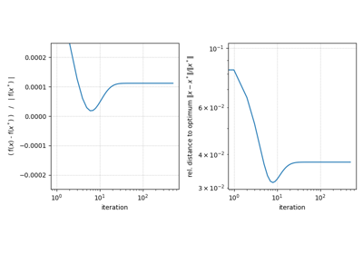
606 if track_cost:
607     fig2, ax2 = plt.subplots(1, 3, figsize=(12, 4), tight_layout=True)
608     for i in range(2):
609         ax2[i].plot(cost_pdhg, ".-", label="PDHG")
610         ax2[i].plot(cost_lmspdhg, ".-", label="LM-SPDHG")
611         ax2[i].grid(ls=":")
612         ax2[i].legend()
613         ax2[i].set_ylim(None, cost_pdhg[10:].max())
614     ax2[1].set_xlim(0, num_iter_spdhg)
615     ax2[2].plot(psnr_lmspdhg, ".-")
616     ax2[2].grid(ls=":")
617     for axx in ax2.ravel():
618         axx.set_xlabel("iteration")
619     ax2[0].set_title("cost", fontsize="medium")
620     ax2[1].set_title("cost (zoom)", fontsize="medium")
621     ax2[2].set_title("PSNR LM-SPDHG vs ref", fontsize="medium")
622     fig2.show()
Related examples