Note
Go to the end to download the full example code.
Non-TOF and TOF projections using a modularized (block) PET scanner geometry
In this example, we show how to perform non-TOF and TOF projections using a PET scanner consisting of multiple block modules where each block module consists of a regular grid of LOR endpoints.
Tip
parallelproj is python array API compatible meaning it supports different
array backends (e.g. numpy, cupy, torch, …) and devices (CPU or GPU).
Choose your preferred array API xp and device dev below.
19 import array_api_compat.numpy as xp
20
21 # import array_api_compat.cupy as xp
22 # import array_api_compat.torch as xp
23
24 import parallelproj
25 import matplotlib.pyplot as plt
26 import math
27
28 # choose a device (CPU or CUDA GPU)
29 if "numpy" in xp.__name__:
30     # using numpy, device must be cpu
31     dev = "cpu"
32 elif "cupy" in xp.__name__:
33     # using cupy, only cuda devices are possible
34     dev = xp.cuda.Device(0)
35 elif "torch" in xp.__name__:
36     # using torch valid choices are 'cpu' or 'cuda'
37     dev = "cuda"
input paraters
42 # grid shape of LOR endpoints forming a block module
43 block_shape = (3, 2, 2)
44 # spacing between LOR endpoints in a block module
45 block_spacing = (1.5, 1.2, 1.7)
46 # radius of the scanner
47 scanner_radius = 10
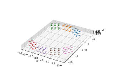
Setup of a modularized PET scanner geometry
We define 7 block modules arranged in a circle with a radius of 10. The arangement follows a regular polygon with 12 sides, leaving some of the sides empty. Note that all block modules must be identical, but can be anywhere in space. The location of a block module can be changed using an affine transformation matrix.
59 mods = []
60
61 delta_phi = 2 * xp.pi / 12
62
63 # setup an affine transformation matrix to translate the block modules from the
64 # center to the radius of the scanner
65 aff_mat_trans = xp.eye(4, device=dev)
66 aff_mat_trans[1, -1] = scanner_radius
67
68 for phi in [
69     -delta_phi,
70     0,
71     delta_phi,
72     5 * delta_phi,
73     6 * delta_phi,
74     7 * delta_phi,
75 ]:
76     # setup an affine transformation matrix to rotate the block modules around the center
77     # (of the "2" axis)
78     aff_mat_rot = xp.asarray(
79         [
80             [math.cos(phi), -math.sin(phi), 0, 0],
81             [math.sin(phi), math.cos(phi), 0, 0],
82             [0, 0, 1, 0],
83             [0, 0, 0, 1],
84         ]
85     )
86     mods.append(
87         parallelproj.BlockPETScannerModule(
88             xp,
89             dev,
90             block_shape,
91             block_spacing,
92             affine_transformation_matrix=(aff_mat_rot @ aff_mat_trans),
93         )
94     )
95
96 # create the scanner geometry from a list of identical block modules at
97 # different locations in space
98 scanner = parallelproj.ModularizedPETScannerGeometry(mods)
Setup of a LOR descriptor consisting of block pairs
Once the geometry of the LOR endpoints is defined, we can define the LORs by specifying which block pairs are in coincidence and for “valid” LORs. To do this, we have manually define a list containing pairs of block numbers. Here, we define 9 block pairs. Note that more pairs would be possible.
109 lor_desc = parallelproj.EqualBlockPETLORDescriptor(
110     scanner,
111     xp.asarray(
112         [
113             [0, 3],
114             [0, 4],
115             [0, 5],
116             [1, 3],
117             [1, 4],
118             [1, 5],
119             [2, 3],
120             [2, 4],
121             [2, 5],
122         ]
123     ),
124 )
Setup of a non-TOF projector
Now that the LOR descriptor is defined, we can setup the projector.
132 img_shape = (28, 20, 3)
133 voxel_size = (0.5, 0.5, 1.0)
134 img = xp.ones(img_shape, dtype=xp.float32, device=dev)
135
136 proj = parallelproj.EqualBlockPETProjector(lor_desc, img_shape, voxel_size)
137 assert proj.adjointness_test(xp, dev)
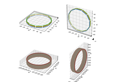
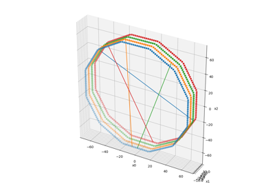
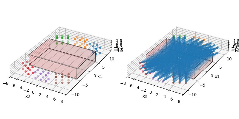
Visualize the projector geometry and all LORs
142 fig = plt.figure(figsize=(8, 4), tight_layout=True)
143 ax0 = fig.add_subplot(121, projection="3d")
144 ax1 = fig.add_subplot(122, projection="3d")
145 proj.show_geometry(ax0)
146 proj.show_geometry(ax1)
147 lor_desc.show_block_pair_lors(ax1, block_pair_nums=None, color=plt.cm.tab10(0))
148 fig.show()
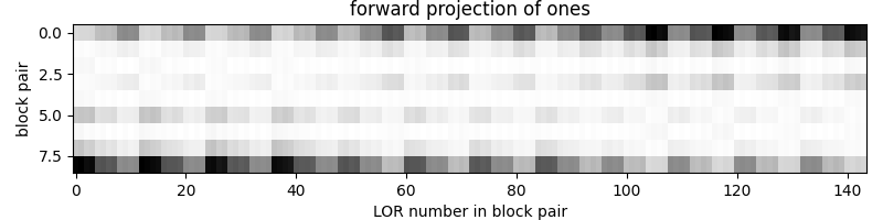
Forward project an image full of ones. The forward projection has the shape (num_block_pairs, num_lors_per_block_pair)
155 img_fwd = proj(img)
156 print(img_fwd.shape)
(9, 144)
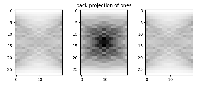
Backproject a “histogram” full of ones (“sensitivity image” when attenuation and normalization are ignored)
162 ones_back = proj.adjoint(xp.ones(proj.out_shape, dtype=xp.float32, device=dev))
163 print(ones_back.shape)
(28, 20, 3)
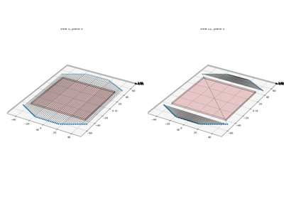
Visualize the forward and backward projection results
168 fig3, ax3 = plt.subplots(figsize=(8, 2), tight_layout=True)
169 ax3.imshow(parallelproj.to_numpy_array(img_fwd), cmap="Greys", aspect=3.0)
170 ax3.set_xlabel("LOR number in block pair")
171 ax3.set_ylabel("block pair")
172 ax3.set_title("forward projection of ones")
173 fig3.show()
174
175 fig4, ax4 = plt.subplots(1, 3, figsize=(7, 3), tight_layout=True)
176 vmin = float(xp.min(ones_back))
177 vmax = float(xp.max(ones_back))
178 for i in range(3):
179     ax4[i].imshow(
180         parallelproj.to_numpy_array(ones_back[:, :, i]),
181         vmin=vmin,
182         vmax=vmax,
183         cmap="Greys",
184     )
185 ax4[1].set_title("back projection of ones")
186 fig4.show()
Setup of a TOF projector
Now that the LOR descriptor is defined, we can setup the projector.
194 proj_tof = parallelproj.EqualBlockPETProjector(lor_desc, img_shape, voxel_size)
195 proj_tof.tof_parameters = parallelproj.TOFParameters(
196     num_tofbins=27, tofbin_width=0.8, sigma_tof=2.0, num_sigmas=3.0
197 )
198
199 assert proj_tof.adjointness_test(xp, dev)
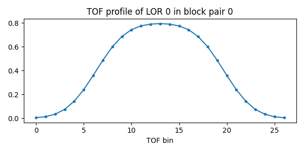
TOF forward project an image full of ones. The forward projection has the shape (num_block_pairs, num_lors_per_block_pair, num_tofbins)
205 img_fwd_tof = proj_tof(img)
206 print(img_fwd_tof.shape)
(9, 144, 27)
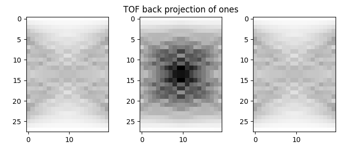
TOF backproject a “TOF histogram” full of ones (“sensitivity image” when attenuation and normalization are ignored)
212 ones_back_tof = proj_tof.adjoint(
213     xp.ones(proj_tof.out_shape, dtype=xp.float32, device=dev)
214 )
215 print(ones_back_tof.shape)
(28, 20, 3)
Visualize the forward and backward projection results
220 fig5, ax5 = plt.subplots(figsize=(6, 3), tight_layout=True)
221 ax5.plot(parallelproj.to_numpy_array(img_fwd_tof[0, 0, :]), ".-")
222 ax5.set_xlabel("TOF bin")
223 ax5.set_title("TOF profile of LOR 0 in block pair 0")
224 fig5.show()
225
226 fig6, ax6 = plt.subplots(1, 3, figsize=(7, 3), tight_layout=True)
227 vmin = float(xp.min(ones_back_tof))
228 vmax = float(xp.max(ones_back_tof))
229 for i in range(3):
230     ax6[i].imshow(
231         parallelproj.to_numpy_array(ones_back_tof[:, :, i]),
232         vmin=vmin,
233         vmax=vmax,
234         cmap="Greys",
235     )
236 ax6[1].set_title("TOF back projection of ones")
237 fig6.show()
Total running time of the script: (0 minutes 1.674 seconds)
Related examples