Michelograms and axial sinogram compression

A Michelogram is a diagram of which ring pairs (s, e) form valid coincidences in a cylindrical PET scanner, and how they are grouped into sinogram planes under Siemens / STIR axial compression conventions. Ring pairs are sorted by segment (a function of the ring difference rd = e - s) and, within each segment, by axial midpoint s + e.

This example introduces

• Michelogram – captures the segment / axial-position layout in pure integer space, independently of any scanner geometry;

• SinogramAxialCompressionOperator – the linear operator that uses a Michelogram to compress a span-1 sinogram into a higher-span sinogram by summing the ring-pair sinograms that fold into the same compressed plane.

import numpy as np
import matplotlib.pyplot as plt

import parallelproj.pet_scanners
import parallelproj.pet_lors
import parallelproj.projectors
from parallelproj import to_numpy_array

from parallelproj._examples_utils import suggest_array_backend_and_device, show_vol_cuts

# To use a specific backend and/or device, replace the None arguments, e.g.:
#   xp, dev = suggest_array_backend_and_device(backend="numpy", dev="cpu") or by setting xp and dev manually
xp, dev = suggest_array_backend_and_device(None, None)

Using array API: array_api_compat.torch, device: cpu

A Michelogram, standalone

A Michelogram is built from three integers:

• num_rings – the number of detector rings,

• max_ring_difference – the maximum |e - s| considered,

• span – an odd axial compression factor (1 = no compression).

It knows nothing about ring z-positions or scanner radius – it is a combinatorial object describing the (segment, axial midpoint) layout of sinogram planes. Each point in the Michelogram plot is one valid ring pair (start_ring, end_ring), coloured by |segment|; numerals annotate the resulting sinogram plane index.

num_rings = 13

m_span1 = parallelproj.pet_lors.Michelogram(
    num_rings=num_rings,
    max_ring_difference=num_rings - 1,
    span=1,
)

print(repr(m_span1))
print(f"num_planes       = {m_span1.num_planes}")
print(f"max_multiplicity = {m_span1.max_multiplicity}")

fig, ax = plt.subplots(figsize=(9, 9), tight_layout=True)
m_span1.show(ax, plane_index_fontsize=8)
fig.show()

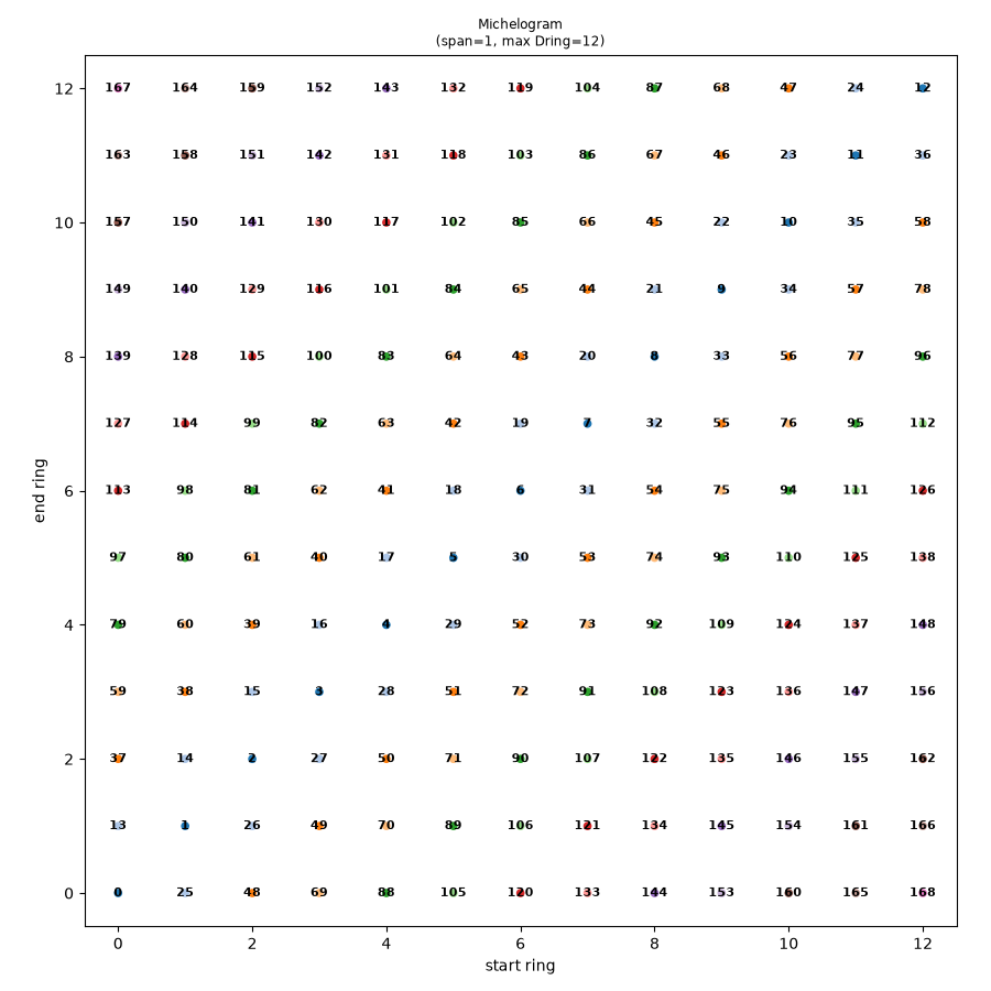
Michelogram(num_rings=13, max_ring_difference=12, span=1)
num_planes       = 169
max_multiplicity = 1

Effect of span and max_ring_difference

Increasing the span merges ring pairs that share both a segment and an axial midpoint into one sinogram plane. In the Michelogram plot, merged ring pairs are connected by thin grey merge lines – visually, each grey line collapses into one plane index.

Restricting the max_ring_difference removes the outer segments entirely, shrinking the diagonal band of valid ring pairs.

configs = [
    (1, num_rings - 1),  # span=1, all ring differences
    (3, num_rings - 1),  # span=3, all ring differences
    (5, num_rings - 1),  # span=5, all ring differences
    (5, 5),  # span=5, max_ring_difference restricted
]

fig, axes = plt.subplots(2, 2, figsize=(14, 14), tight_layout=True)
for ax, (span, mrd) in zip(axes.flat, configs):
    m = parallelproj.pet_lors.Michelogram(
        num_rings=num_rings,
        max_ring_difference=mrd,
        span=span,
    )
    m.show(ax, plane_index_fontsize=7)
    ax.set_title(
        f"span={span}, max_ring_difference={mrd}\n"
        f"-> num_planes = {m.num_planes}, "
        f"max_multiplicity = {m.max_multiplicity}",
        fontsize="medium",
    )
fig.show()

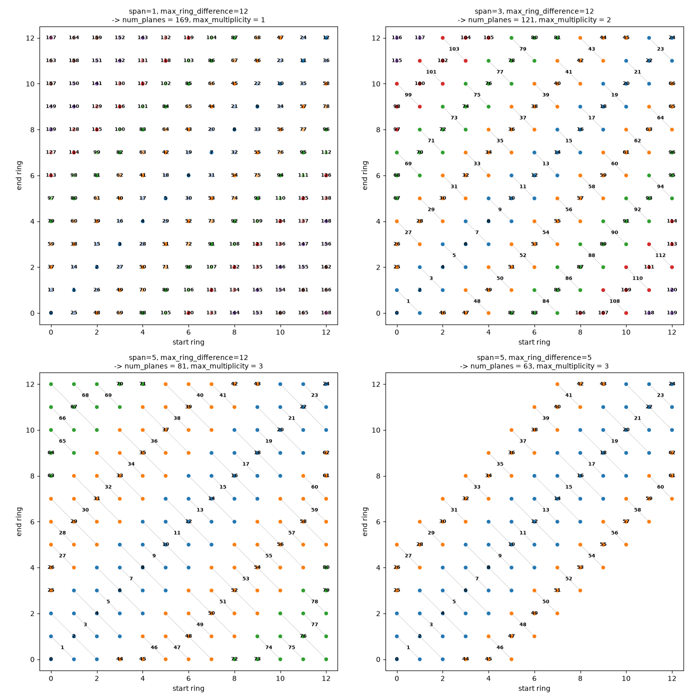
Axial Compression of span-1 sinograms to a span > 1

SinogramAxialCompressionOperator takes a span-1 LOR descriptor and a target odd span, and produces a linear operator that maps a span-1 sinogram to a span-target_span sinogram via

\[y_n = \sum_{p_1 \,\in\, \mathcal{G}(n)} x_{p_1}\,,\]

where \(\mathcal{G}(n)\) is the set of span-1 plane indices that fold into target plane \(n\). Its transpose replicates each output value back to every input plane that contributed to it.

To see the operator in action, we set up a small 5-ring scanner, build a span-1 projector, forward-project a small Gaussian phantom, then compress the resulting span-1 sinogram to span 5.

num_rings_small = 5
target_span = 5

scanner_small = parallelproj.pet_scanners.RegularPolygonPETScannerGeometry(
    xp,
    dev,
    radius=65.0,
    num_sides=12,
    num_lor_endpoints_per_side=4,
    lor_spacing=4.0,
    ring_positions=xp.linspace(-4, 4, num_rings_small, device=dev),
    symmetry_axis=2,
)

# span-1 descriptor (no ring-difference constraint)
lor_s1 = parallelproj.pet_lors.RegularPolygonPETLORDescriptor(
    scanner_small,
    parallelproj.pet_lors.Michelogram(
        scanner_small.num_rings,
        max_ring_difference=num_rings_small - 1,
        span=1,
    ),
    radial_trim=10,
)

# span-1 forward projector
img_shape = (32, 32, 11)
voxel_size = (2.0, 2.0, 1.0)

proj_s1 = parallelproj.projectors.RegularPolygonPETProjector(
    lor_s1, img_shape=img_shape, voxel_size=voxel_size
)

# axial compression operator (span 1 -> span target_span)
op = parallelproj.pet_lors.SinogramAxialCompressionOperator(
    lor_s1, target_span=target_span
)

print(op)
print(f"span-1 sinogram shape: {proj_s1.out_shape}")
print(f"span-{target_span} sinogram shape: {op.out_shape}")

SinogramAxialCompressionOperator(target_span=5, mode='sum', num_planes: 25 -> 15, max_multiplicity=3)
span-1 sinogram shape: (27, 24, 25)
span-5 sinogram shape: (27, 24, 15)

A tiny 3-D Gaussian phantom, centered off-axis at world coordinates (x, y, z) = (0, 10, 0) mm with isotropic sigma = 4 mm. The image lives in numpy; we convert to xp for the projector.

ii, jj, kk = np.meshgrid(
    np.arange(img_shape[0]),
    np.arange(img_shape[1]),
    np.arange(img_shape[2]),
    indexing="ij",
)
x_w = (ii - (img_shape[0] - 1) / 2) * voxel_size[0]
y_w = (jj - (img_shape[1] - 1) / 2) * voxel_size[1]
z_w = (kk - (img_shape[2] - 1) / 2) * voxel_size[2]
phantom_np = np.exp(
    -((x_w - 0.0) ** 2 + (y_w - 10.0) ** 2 + (z_w - 0.0) ** 2) / (2 * 4.0**2)
).astype(np.float32)

phantom = xp.asarray(phantom_np, device=dev)

# Forward-project at span 1, then axially compress to span ``target_span``.
sino_s1 = proj_s1(phantom)
sino_sn = op(sino_s1)

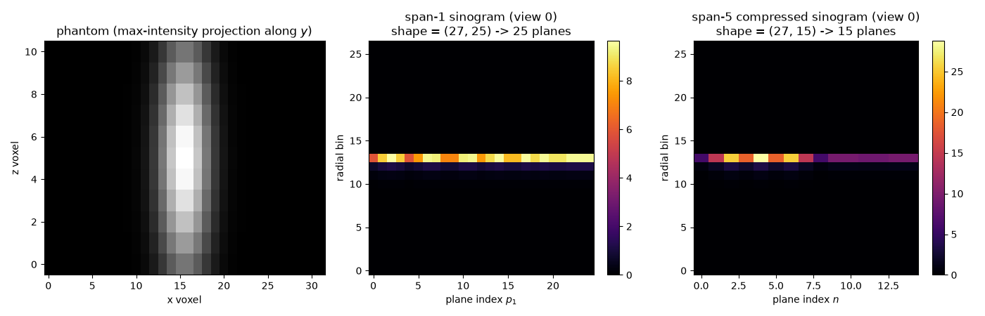
Visualise: a maximum-intensity projection of the 3-D phantom along the y axis (so the axial structure is visible), and the resulting span-1 and span-target_span sinograms for the same view. The plane axis of each sinogram encodes axial position; compressing reduces the number of plane bins (and increases per-bin values because of the summation).

view_idx = 0
s1_np = to_numpy_array(sino_s1)[:, view_idx, :]
sn_np = to_numpy_array(sino_sn)[:, view_idx, :]

fig, axes = plt.subplots(1, 3, figsize=(14, 4.5), tight_layout=True)

axes[0].imshow(phantom_np.max(axis=1).T, origin="lower", cmap="gray", aspect="auto")
axes[0].set_title("phantom (max-intensity projection along $y$)")
axes[0].set_xlabel("x voxel")
axes[0].set_ylabel("z voxel")

im1 = axes[1].imshow(s1_np, origin="lower", cmap="inferno", aspect="auto")
axes[1].set_title(
    f"span-1 sinogram (view {view_idx})\n"
    f"shape = {s1_np.shape} -> {op.num_planes_in} planes"
)
axes[1].set_xlabel("plane index $p_1$")
axes[1].set_ylabel("radial bin")
fig.colorbar(im1, ax=axes[1])

im2 = axes[2].imshow(sn_np, origin="lower", cmap="inferno", aspect="auto")
axes[2].set_title(
    f"span-{target_span} compressed sinogram (view {view_idx})\n"
    f"shape = {sn_np.shape} -> {op.num_planes_out} planes"
)
axes[2].set_xlabel("plane index $n$")
axes[2].set_ylabel("radial bin")
fig.colorbar(im2, ax=axes[2])

fig.show()

A direct span-\(S\) projector is not the same as compressing a span-1 sinogram ———————————————————————-

A natural question: instead of forward-projecting at span 1 and then applying the compression operator, can we just build a span-\(S\) RegularPolygonPETProjector directly? The answer is “yes, but they are not interchangeable”.

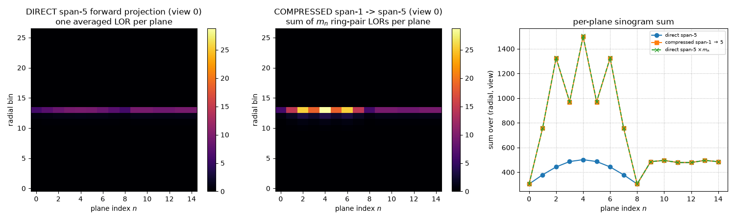
A span-\(S\) descriptor uses one averaged LOR per compressed plane (the geometric average of the constituent ring-pair LORs), so the direct projector traces one ray per output plane:

\[(\text{direct span-}S)_n \;=\; \int_{\,\text{LOR}_{\,\text{avg}}(n)} f(x)\, dx\,.\]

The compression operator, in contrast, sums every ring-pair line integral that folds into plane \(n\):

\[(\text{compressed})_n \;=\; \sum_{p_1 \,\in\, \mathcal{G}(n)} \int_{\,\text{LOR}(p_1)} f(x)\, dx\, \;\approx\; m_n \cdot (\text{direct span-}S)_n\,,\]

where \(m_n\) is the plane multiplicity. The compressed result therefore overcounts by a factor of \(m_n\) relative to the direct span-\(S\) projection.

Practical consequence. In a real reconstruction with spanned data one typically uses the (much faster) span-\(S\) projector – but the per-plane multiplicities must then be folded into the multiplicative sensitivity / normalisation sinogram so that the data model stays consistent.

lor_sn_direct = parallelproj.pet_lors.RegularPolygonPETLORDescriptor(
    scanner_small,
    parallelproj.pet_lors.Michelogram(
        scanner_small.num_rings,
        max_ring_difference=num_rings_small - 1,
        span=target_span,
    ),
    radial_trim=10,
)
proj_sn_direct = parallelproj.projectors.RegularPolygonPETProjector(
    lor_sn_direct, img_shape=img_shape, voxel_size=voxel_size
)

sino_sn_direct = proj_sn_direct(phantom)

Visualise: the direct span-\(S\) sinogram, the compressed one, and a per-plane sum comparison that makes the \(m_n\) factor explicit.

sn_direct_np = to_numpy_array(sino_sn_direct)[:, view_idx, :]
mult_np = to_numpy_array(op.plane_multiplicity)
direct_per_plane = to_numpy_array(sino_sn_direct).sum(axis=(0, 1))
compressed_per_plane = to_numpy_array(sino_sn).sum(axis=(0, 1))

fig, axes = plt.subplots(1, 3, figsize=(15, 4.5), tight_layout=True)

vmax_panels = float(max(sn_direct_np.max(), sn_np.max()))

im_a = axes[0].imshow(
    sn_direct_np, origin="lower", cmap="inferno", vmax=vmax_panels, aspect="auto"
)
axes[0].set_title(
    f"DIRECT span-{target_span} forward projection (view {view_idx})\n"
    "one averaged LOR per plane"
)
axes[0].set_xlabel("plane index $n$")
axes[0].set_ylabel("radial bin")
fig.colorbar(im_a, ax=axes[0])

im_b = axes[1].imshow(
    sn_np, origin="lower", cmap="inferno", vmax=vmax_panels, aspect="auto"
)
axes[1].set_title(
    f"COMPRESSED span-1 -> span-{target_span} (view {view_idx})\n"
    "sum of $m_n$ ring-pair LORs per plane"
)
axes[1].set_xlabel("plane index $n$")
axes[1].set_ylabel("radial bin")
fig.colorbar(im_b, ax=axes[1])

axes[2].plot(direct_per_plane, "o-", label=f"direct span-{target_span}")
axes[2].plot(
    compressed_per_plane, "s-", label=f"compressed span-1 $\\to$ {target_span}"
)
axes[2].plot(
    direct_per_plane * mult_np,
    "x--",
    label=f"direct span-{target_span} $\\times\\, m_n$",
)
axes[2].set_xlabel("plane index $n$")
axes[2].set_ylabel("sum over (radial, view)")
axes[2].set_title("per-plane sinogram sum")
axes[2].legend(fontsize="x-small")
axes[2].grid(True, ls=":")

fig.show()

Ratio of per-plane sums vs multiplicity

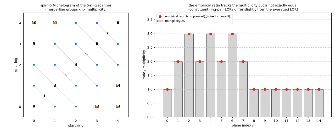
Plotting the empirical ratio \((\text{compressed})_n / (\text{direct span-}S)_n\) against the plane multiplicity \(m_n\) makes the relationship explicit. The two are close but not identical: every ring-pair LOR within a compressed group has its own length and orientation, so its line integral through the phantom differs slightly from the integral through the single averaged LOR that the direct span-\(S\) projector uses. How “close” depends on (a) how strongly the constituent LORs differ within a compressed group and (b) how much axial structure the phantom has where those LORs diverge.

We plot the span-\(S\) Michelogram alongside the ratio so the multiplicity can be read off directly: each merge-line group (or each isolated dot) is one output plane, and the number of ring pairs in that group is \(m_n\).

# guard against divide-by-zero for planes that don't intersect the phantom
threshold = 1e-6 * float(direct_per_plane.max())
mask_valid = direct_per_plane > threshold
ratio = np.full_like(direct_per_plane, np.nan, dtype=float)
ratio[mask_valid] = compressed_per_plane[mask_valid] / direct_per_plane[mask_valid]

fig, axes = plt.subplots(
    1, 2, figsize=(14, 5.5), tight_layout=True, gridspec_kw={"width_ratios": [1, 1.4]}
)

# --- left: the span-S Michelogram of the 5-ring scanner ---
op.out_lor_descriptor.michelogram.show(axes[0], plane_index_fontsize=11)
axes[0].set_title(
    f"span-{target_span} Michelogram of the 5-ring scanner\n"
    f"(merge-line groups <-> multiplicity)",
    fontsize="medium",
)

# --- right: empirical ratio vs multiplicity bars ---
n_idx = np.arange(op.num_planes_out)
axes[1].bar(
    n_idx,
    mult_np,
    color="lightgray",
    edgecolor="black",
    lw=0.5,
    label="multiplicity $m_n$",
)
axes[1].plot(
    n_idx[mask_valid],
    ratio[mask_valid],
    "o",
    color="C3",
    ms=7,
    label=r"empirical ratio "
    r"$(\mathrm{compressed})_n / (\mathrm{direct\;span-}S)_n$",
)
axes[1].set_xlabel("plane index $n$")
axes[1].set_ylabel("ratio / multiplicity")
axes[1].set_title(
    "the empirical ratio tracks the multiplicity but is not exactly equal\n"
    "(constituent ring-pair LORs differ slightly from the averaged LOR)",
    fontsize="medium",
)
axes[1].set_xticks(n_idx)
axes[1].set_ylim(0, max(float(mult_np.max()), float(np.nanmax(ratio))) * 1.25)
axes[1].legend(loc="upper left", fontsize="small")
axes[1].grid(True, ls=":", axis="y")

fig.show()

GE-style layout

GE-style scanners use a mixed axial layout that does not correspond to a single (odd) span. Select it with layout=MichelogramLayout.GE or the Michelogram.ge() convenience constructor; span is then ignored and Michelogram.span returns None. Using the usual segment (theta) / ring-difference (dZ) terminology:

• segment 0 collects ring differences dZ = {-1, 0, +1} – the +/-1 cross planes are summed into virtual direct planes at the intermediate axial positions (exactly like a Siemens span-3 segment 0);

• every oblique segment +/-k collects the ring-difference pair {+/-2k, +/-(2k+1)} without combination, laid out as a staircase.

Segments are ordered 0, +1, -1, +2, -2, ... (also known as “span 2” in STIR). Pick num_rings and max_ring_difference to match the GE scanner of interest.

m_ge = parallelproj.pet_lors.Michelogram.ge(num_rings=9, max_ring_difference=8)
print(
    f"GE layout: span={m_ge.span}, num_planes={m_ge.num_planes}, "
    f"max_multiplicity={m_ge.max_multiplicity}"
)

fig_ge, ax_ge = plt.subplots(1, 1, figsize=(5.5, 5.5), tight_layout=True)
m_ge.show(ax_ge, plane_index_fontsize=7)
ax_ge.set_title(
    "GE layout Michelogram (9 rings)\n"
    "segment 0 = dZ{-1,0,1} (cross planes merged), oblique segments = dZ pairs",
    fontsize="small",
)
fig_ge.show()

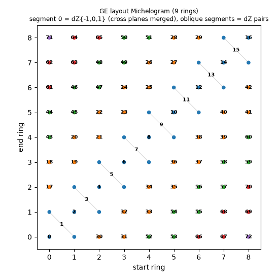
GE layout: span=None, num_planes=73, max_multiplicity=2

Segment ordering: positive-first vs negative-first

Within the sinogram, segment 0 always comes first; the remaining oblique segments are laid out as \(\pm k\) pairs. The SegmentOrder enum controls which member of each pair precedes the other:

• SegmentOrder.POSITIVE_FIRST (default) -> 0, +1, -1, +2, -2, ...

• SegmentOrder.NEGATIVE_FIRST -> 0, -1, +1, -2, +2, ...

This is a pure permutation of the sinogram planes: the ring pairs, the per-plane multiplicities and the segment numbering are all unchanged – only the plane index assigned to each (segment, axial midpoint) group differs. It applies to both the STANDARD and GE layouts and is set on the Michelogram (and forwarded by Michelogram.ge() and SinogramAxialCompressionOperator’s target_segment_order argument).

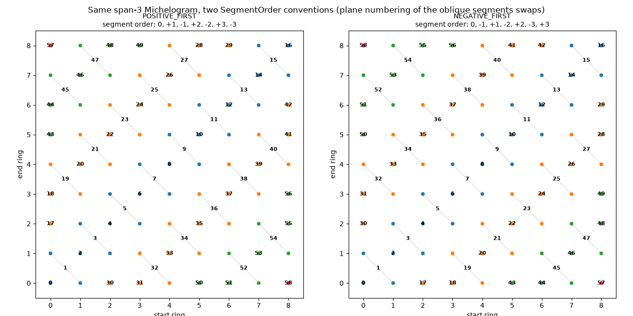
Below we build the same Michelogram under both orderings. The plane-index numerals in segment 0 are identical, but the numbering of the oblique segments swaps: read off how the +k and -k staircases trade their index ranges. We do this once for a Siemens-style span-3 layout and once for the GE layout, since the ordering knob applies to both.

SegmentOrder = parallelproj.pet_lors.SegmentOrder


def _show_segment_order_pair(make_michelogram, suptitle):
    """Draw a POSITIVE_FIRST vs NEGATIVE_FIRST Michelogram pair.

    ``make_michelogram(order)`` returns a :class:`.Michelogram` built with the
    given :class:`.SegmentOrder`.
    """
    fig, axes = plt.subplots(1, 2, figsize=(13, 6.5), tight_layout=True)
    for ax, order in zip(
        axes, (SegmentOrder.POSITIVE_FIRST, SegmentOrder.NEGATIVE_FIRST)
    ):
        m_order = make_michelogram(order)
        m_order.show(ax, plane_index_fontsize=8)
        # de-duplicated, order-preserving segment sequence for the title
        seen: list[int] = []
        for s in (int(v) for v in to_numpy_array(m_order.plane_segment)):
            if s not in seen:
                seen.append(s)
        ax.set_title(
            f"{order.name}\nsegment order: "
            + ", ".join(f"{s:+d}" if s != 0 else "0" for s in seen),
            fontsize="medium",
        )
    fig.suptitle(suptitle, fontsize="large")
    fig.show()


# Siemens-style span-3 layout under both orderings
_show_segment_order_pair(
    lambda order: parallelproj.pet_lors.Michelogram(
        num_rings=9,
        max_ring_difference=8,
        span=3,
        segment_order=order,
    ),
    "Same span-3 Michelogram, two SegmentOrder conventions "
    "(plane numbering of the oblique segments swaps)",
)

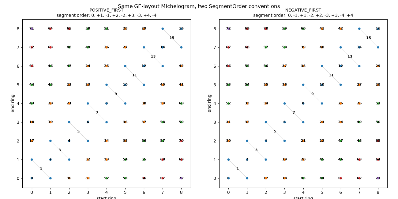
The same knob works for the GE layout. Here segment 0 already folds the dZ = {-1, 0, +1} cross planes into virtual direct planes, and each oblique segment +/-k is a {+/-2k, +/-(2k+1)} staircase; the segment_order only decides whether +k or -k is numbered first. Michelogram.ge forwards the argument, so no layout= is needed.

_show_segment_order_pair(
    lambda order: parallelproj.pet_lors.Michelogram.ge(
        num_rings=9,
        max_ring_difference=8,
        segment_order=order,
    ),
    "Same GE-layout Michelogram, two SegmentOrder conventions",
)

Projecting only a subset of segments with SinogramSegmentSelectionOperator

You may want the full michelogram geometry but only need to project / reconstruct a few segments – e.g. the direct segment and the first oblique ones – to reduce the number of planes. SinogramSegmentSelectionOperator takes the full (span-1 here) descriptor and a list of segments to keep. It builds a matching restricted_lor_descriptor (use it to construct the projector for the restricted sinogram) and, as a linear operator, gathers the selected planes out of a full sinogram (forward) and scatters them back into a zero-filled full sinogram (adjoint).

We reuse the span-1 descriptor lor_s1, its projector proj_s1 and the full sinogram sino_s1 built further above.

# (1) full descriptor + projector + full sinogram already exist:
#     lor_s1, proj_s1, sino_s1 = proj_s1(phantom)

# (2) selection operator keeping segments 0, -1 and +1
selected_segments = [0, -1, 1]
seg_sel = parallelproj.pet_lors.SinogramSegmentSelectionOperator(
    lor_s1, segments=selected_segments
)
print(seg_sel)
print(f"full sinogram planes:       {seg_sel.num_planes_in}")
print(f"restricted sinogram planes: {seg_sel.num_planes_out}")

# (3) build the projector for the restricted geometry straight from the operator
proj_restricted = parallelproj.projectors.RegularPolygonPETProjector(
    seg_sel.restricted_lor_descriptor, img_shape=img_shape, voxel_size=voxel_size
)

# the restricted version of the full sinogram from step (1)
sino_restricted = seg_sel(sino_s1)

# (4) back-project the restricted sinogram with the restricted projector,
#     and -- for reference -- the full sinogram with the full projector
back_restricted = proj_restricted.adjoint(sino_restricted)
back_full = proj_s1.adjoint(sino_s1)

SinogramSegmentSelectionOperator(segments=[0, 1, -1], num_planes: 25 -> 13)
full sinogram planes:       25
restricted sinogram planes: 13

Consistency check: projecting the phantom directly with the restricted projector must equal gathering the selected planes out of the full forward projection (same geometry, same plane ordering – just fewer planes).

sino_restricted_direct = proj_restricted(phantom)
max_abs_diff = float(xp.max(xp.abs(sino_restricted_direct - sino_restricted)))
print(f"max |restricted_direct - gather(full)| = {max_abs_diff:.3e}")

max |restricted_direct - gather(full)| = 0.000e+00

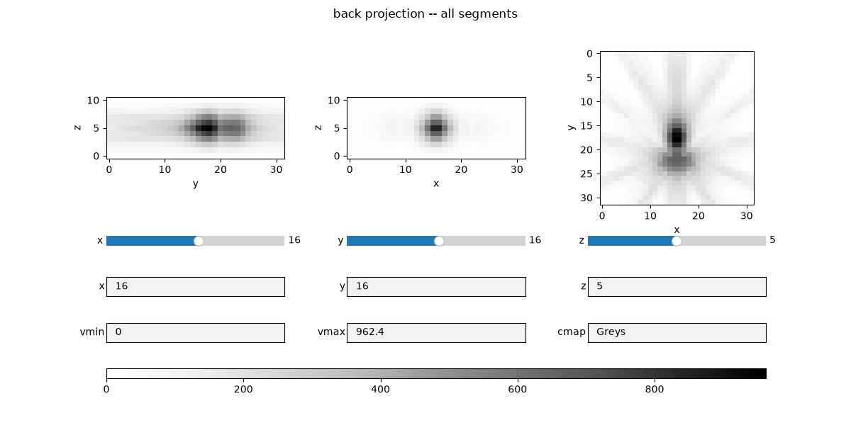
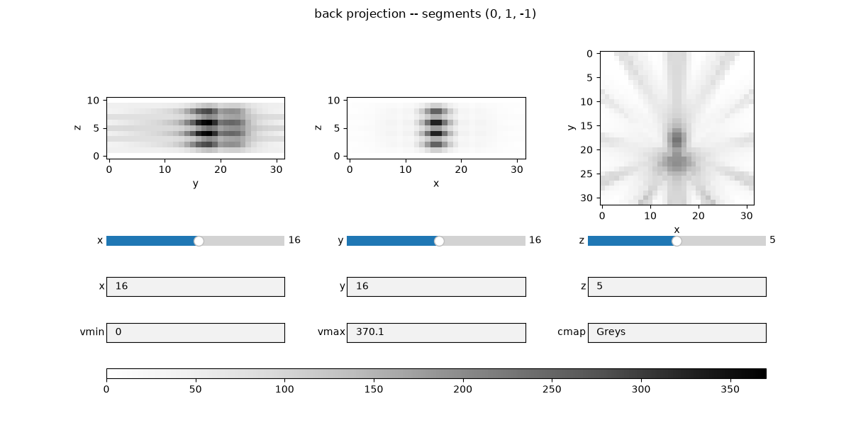
Visualise the two back-projections. The restricted back projection uses only the selected segments’ LORs, so it is a (blurrier, fewer-plane-contribution) approximation of the full back projection.

fig_bp_full, _, _ = show_vol_cuts(
    back_full, fig_title="back projection -- all segments"
)
fig_bp_full.show()

fig_bp_restr, _, _ = show_vol_cuts(
    back_restricted,
    fig_title=f"back projection -- segments {seg_sel.segments}",
)
fig_bp_restr.show()

• 
•