Penalised transmission reconstruction (MAPTR) with an edge-preserving prior

This example adds an edge-preserving smoothing prior to the ordered-subset transmission reconstruction of 01_os_mltr_svrg.py (MAPTR – maximum a posteriori transmission reconstruction). We now minimise the penalised objective

\[\Phi(\mu) = -L(\mu) + \beta R(\mu)\]

\[L(\mu) = \sum_i y_i \ln \bar{y}_i (\mu) - \bar{y}_i (\mu), \qquad \bar{y}_i (\mu) = \bar{z}_i (\mu) + s_i, \qquad \bar{z}_i (\mu) = b_i e^{-(P \mu)_i},\]

with a log-cosh roughness penalty on the nearest-neighbour finite differences \(G\mu\),

\[R(\mu) = \delta \sum_d \sum_j \log\cosh\!\left(\frac{(G\mu)_{d,j}}{\delta}\right), \qquad \nabla R = G^T \tanh(G\mu/\delta).\]

The log-cosh penalty is quadratic for differences \(\ll \delta\) (smooths noise) and linear for differences \(\gg \delta\) (preserves edges). We set \(\delta = \mu_{\text{water}}/2\), so the dense-insert jumps (several times \(\mu_{\text{water}}\)) sit in the edge-preserving linear regime while background noise is smoothed.

Preconditioner – the transmission “harmonic-mean” analogue. In emission MAP-EM one combines the EM step \(x/A^T\mathbf 1\) with the prior curvature; that is the harmonic mean of the two step sizes, i.e. the reciprocal of the sum of curvatures. Here the MLTR denominator \(P^T[(P\mathbf 1)\,\bar z^2/\bar y]\) is exactly the separable diagonal majorant of the data Hessian (the analogue of \(A^T\mathbf 1 / x\)), so the penalised preconditioner is

\[D(\mu) = \frac{1}{\;P^T\!\left[(P\mathbf 1)\,\bar z^2/\bar y\right] + \beta\,\kappa/\delta\;},\]

where \(\beta\,\kappa/\delta\) (with \(\kappa = \operatorname{diag}(G^TG) \approx 2\,n_\text{dim}\)) is the log-cosh prior’s maximal curvature – a valid diagonal majorant, since \(\tfrac{d^2}{dz^2}\delta\log\cosh(z/\delta) = \tfrac1\delta\operatorname{sech}^2 \le \tfrac1\delta\).

The subset algorithms of 01_os_mltr_svrg.py are run, now on the penalised objective, with a converged L-BFGS-B reference:

• OS-MLTR – one subset per update; the prior is split beta/m per subset so the \(m\) subset contributions sum to the full penalty.

• SVRG – the data term is variance-reduced across subsets; the cheap, deterministic prior gradient \(\beta\nabla R(\mu)\) is added in full at every inner step.

Note

Each OS-MLTR epoch is one full data pass; an SVRG epoch is roughly 1.5 (anchor + subset sweep), so the epoch axis understates SVRG’s cost by about a factor of 1.5.

from __future__ import annotations

from copy import copy

import matplotlib.pyplot as plt
import numpy as np
from scipy.optimize import minimize

import parallelproj.operators
import parallelproj.pet_lors
import parallelproj.pet_scanners
import parallelproj.projectors
from parallelproj import Array, to_numpy_array
from parallelproj.functions import C2AffineObjective, LogCosh


from parallelproj._examples_utils import (
    elliptic_cylinder_phantom,
    poisson_transmission_terms,
    show_vol_cuts,
)

from parallelproj._examples_utils import suggest_array_backend_and_device

# To use a specific backend and/or device, replace the None arguments, e.g.:
#   xp, dev = suggest_array_backend_and_device(backend="numpy", dev="cpu")
xp, dev = suggest_array_backend_and_device(None, None)

Using array API: array_api_compat.torch, device: cpu

num_epochs = 30  # epochs (full data passes) for the subset algorithms
num_subsets = 28  # number of ordered view subsets (divides the 168 views evenly)
num_lbfgs = 80  # L-BFGS-B iterations for the reference solution
blank_counts = 500.0  # blank scan counts per LOR
scatter_fraction = 0.5  # scatter relative to mean unscattered transmission

mu_water = 0.0096  # 1/mm at 511 keV
beta = 2e2  # prior weight
# log-cosh transition scale: edges (dense inserts) >> delta are preserved,
# background noise << delta is smoothed
delta = mu_water / 2

Scanner, non-TOF projector, and ground-truth attenuation image

num_rings = 3
ring_spacing = 5.3  # mm, axial distance between rings
scanner = parallelproj.pet_scanners.RegularPolygonPETScannerGeometry(
    xp,
    dev,
    radius=300.0,
    num_sides=56,
    num_lor_endpoints_per_side=6,
    lor_spacing=5.3,
    # rings centred on the origin, spacing = ring_spacing -> [-5.3, 0, 5.3]
    ring_positions=(
        xp.arange(num_rings, dtype=xp.float32, device=dev) - (num_rings - 1) / 2
    )
    * ring_spacing,
    symmetry_axis=2,
)

# transaxial 100 x 100 @ 4 mm; axially one slice per ring (5.3 mm),
# so the image slices are aligned with the ring positions
img_shape = (100, 100, num_rings)
voxel_size = (4.0, 4.0, ring_spacing)

lor_desc = parallelproj.pet_lors.RegularPolygonPETLORDescriptor(
    scanner,
    parallelproj.pet_lors.Michelogram(scanner.num_rings, max_ring_difference=2, span=1),
    radial_trim=10,
    sinogram_order=parallelproj.pet_lors.SinogramSpatialAxisOrder.RVP,
)

proj = parallelproj.projectors.RegularPolygonPETProjector(
    lor_desc, img_shape=img_shape, voxel_size=voxel_size
)

mu_true = mu_water * elliptic_cylinder_phantom(
    xp, dev, image_shape=img_shape, voxel_size=voxel_size
)

# voxels never seen by any LOR must not be updated (their denominator is 0)
fov_mask = proj.fov_mask()

Simulate transmission data

b = xp.full(proj.out_shape, blank_counts, device=dev, dtype=xp.float32)

psi_true = b * xp.exp(-proj(mu_true))
s = xp.full(
    proj.out_shape,
    scatter_fraction * float(xp.mean(psi_true)),
    device=dev,
    dtype=xp.float32,
)

np.random.seed(1)
y = xp.asarray(
    np.random.poisson(to_numpy_array(psi_true + s)),
    device=dev,
    dtype=xp.float32,
)

Prior, data and subset ingredients

The log-cosh prior is built from the finite-difference operator G. reg(mu) and reg.gradient(mu) give \(\beta R\) and \(\beta \nabla R\); prior_curv = beta * kappa / delta is the diagonal curvature majorant entering the preconditioner.

ones_img = xp.ones(proj.in_shape, dtype=xp.float32, device=dev)
P1 = proj(ones_img)

G = parallelproj.operators.FiniteForwardDifference(proj.in_shape)
reg = C2AffineObjective(LogCosh(delta=delta, beta=beta), G)
kappa = 2.0 * len(proj.in_shape)  # diag(G^T G) for forward differences
prior_curv = beta * kappa / delta  # log-cosh max curvature (scalar majorant)

subset_views, subset_slices = lor_desc.get_distributed_views_and_slices(
    num_subsets, len(proj.out_shape)
)

subset_proj = []
for k in range(num_subsets):
    p = copy(proj)
    p.views = subset_views[k]
    subset_proj.append(p)

b_k = [b[subset_slices[k]] for k in range(num_subsets)]
s_k = [s[subset_slices[k]] for k in range(num_subsets)]
y_k = [y[subset_slices[k]] for k in range(num_subsets)]
Pk1 = [subset_proj[k](ones_img) for k in range(num_subsets)]


def neg_logL(mu: Array) -> float:
    """Negative transmission Poisson log-likelihood (float64 accumulation)."""
    ybar = b * xp.exp(-proj(mu)) + s
    return float(xp.sum(xp.astype(ybar - y * xp.log(ybar), xp.float64)))


def penalised_cost(mu: Array) -> float:
    """Penalised objective :math:`\\Phi = -L + \\beta R` (to be minimised)."""
    return neg_logL(mu) + float(reg(mu))


def _safe_ratio(num: Array, denom: Array) -> Array:
    """``num / denom`` where the denominator is positive, 0 else (FOV-safe)."""
    ok = fov_mask & (denom > 0)
    denom_safe = xp.where(ok, denom, xp.ones_like(denom))
    return xp.where(ok, num / denom_safe, xp.zeros_like(num))


def full_grad_and_curv(mu: Array) -> tuple[Array, Array]:
    """Full-data gradient of L and the MLTR curvature denominator."""
    _, grad_sino, curv_sino = poisson_transmission_terms(proj(mu), b, s, y)
    return proj.adjoint(grad_sino), proj.adjoint(P1 * curv_sino)


def subset_grad(mu: Array, k: int) -> Array:
    """Gradient of the subset log-likelihood L_k (no 1/m scaling)."""
    _, grad_sino, _ = poisson_transmission_terms(
        subset_proj[k](mu), b_k[k], s_k[k], y_k[k]
    )
    return subset_proj[k].adjoint(grad_sino)

OS-MLTR (one subset per update; prior split beta/m per subset)

Ascend \(L - \beta R\) with the harmonic-mean preconditioner D = 1 / (data curvature + prior curvature), one subset at a time.

cost: dict[str, np.ndarray] = {}
mu_final: dict[str, Array] = {}

mu = xp.zeros(proj.in_shape, dtype=xp.float32, device=dev)
c = [penalised_cost(mu)]
for ep in range(num_epochs):
    print(f"OS-MLTR    epoch {ep + 1:03}/{num_epochs:03}", end="\r")
    for k in range(num_subsets):
        _, grad_sino, curv_sino = poisson_transmission_terms(
            subset_proj[k](mu), b_k[k], s_k[k], y_k[k]
        )
        num = subset_proj[k].adjoint(grad_sino)
        denom = subset_proj[k].adjoint(Pk1[k] * curv_sino)
        g_pen = num - reg.gradient(mu) / num_subsets
        mu = xp.clip(mu + _safe_ratio(g_pen, denom + prior_curv / num_subsets), 0, None)
    c.append(penalised_cost(mu))
print()
cost["OS-MLTR"] = np.asarray(c)
mu_final["OS-MLTR"] = mu

OS-MLTR    epoch 001/030
OS-MLTR    epoch 002/030
OS-MLTR    epoch 003/030
OS-MLTR    epoch 004/030
OS-MLTR    epoch 005/030
OS-MLTR    epoch 006/030
OS-MLTR    epoch 007/030
OS-MLTR    epoch 008/030
OS-MLTR    epoch 009/030
OS-MLTR    epoch 010/030
OS-MLTR    epoch 011/030
OS-MLTR    epoch 012/030
OS-MLTR    epoch 013/030
OS-MLTR    epoch 014/030
OS-MLTR    epoch 015/030
OS-MLTR    epoch 016/030
OS-MLTR    epoch 017/030
OS-MLTR    epoch 018/030
OS-MLTR    epoch 019/030
OS-MLTR    epoch 020/030
OS-MLTR    epoch 021/030
OS-MLTR    epoch 022/030
OS-MLTR    epoch 023/030
OS-MLTR    epoch 024/030
OS-MLTR    epoch 025/030
OS-MLTR    epoch 026/030
OS-MLTR    epoch 027/030
OS-MLTR    epoch 028/030
OS-MLTR    epoch 029/030
OS-MLTR    epoch 030/030

SVRG (variance-reduced data term + full prior gradient per step)

rng = np.random.default_rng(1)
mu = xp.zeros(proj.in_shape, dtype=xp.float32, device=dev)
c = [penalised_cost(mu)]
for ep in range(num_epochs):
    print(f"SVRG       epoch {ep + 1:03}/{num_epochs:03}", end="\r")

    if ep % 2 == 0:
        anchor = mu
        g_full, denom_full = full_grad_and_curv(anchor)
        gk_anchor = [subset_grad(anchor, k) for k in range(num_subsets)]
        precond = _safe_ratio(xp.ones_like(mu), denom_full + prior_curv)

    for k in rng.permutation(num_subsets):
        # variance-reduced data gradient + full (deterministic) prior gradient
        g_data = g_full + num_subsets * (subset_grad(mu, k) - gk_anchor[k])
        mu = xp.clip(mu + precond * (g_data - reg.gradient(mu)), 0, None)
    c.append(penalised_cost(mu))
print()
cost["SVRG"] = np.asarray(c)
mu_final["SVRG"] = mu

SVRG       epoch 001/030
SVRG       epoch 002/030
SVRG       epoch 003/030
SVRG       epoch 004/030
SVRG       epoch 005/030
SVRG       epoch 006/030
SVRG       epoch 007/030
SVRG       epoch 008/030
SVRG       epoch 009/030
SVRG       epoch 010/030
SVRG       epoch 011/030
SVRG       epoch 012/030
SVRG       epoch 013/030
SVRG       epoch 014/030
SVRG       epoch 015/030
SVRG       epoch 016/030
SVRG       epoch 017/030
SVRG       epoch 018/030
SVRG       epoch 019/030
SVRG       epoch 020/030
SVRG       epoch 021/030
SVRG       epoch 022/030
SVRG       epoch 023/030
SVRG       epoch 024/030
SVRG       epoch 025/030
SVRG       epoch 026/030
SVRG       epoch 027/030
SVRG       epoch 028/030
SVRG       epoch 029/030
SVRG       epoch 030/030

L-BFGS-B reference solution (no subsets) on the penalised objective

n_vox = int(np.prod(proj.in_shape))
cost_lbfgs: list[float] = []  # Phi recorded at every function evaluation


def penalised_cost_and_grad(mu_flat: np.ndarray) -> tuple[float, np.ndarray]:
    m = xp.asarray(mu_flat.reshape(proj.in_shape), dtype=xp.float32, device=dev)
    ybar, grad_sino, _ = poisson_transmission_terms(proj(m), b, s, y)
    val = float(xp.sum(xp.astype(ybar - y * xp.log(ybar), xp.float64))) + float(reg(m))
    # gradient of Phi = -L + beta R; grad_sino is the *ascent* gradient of L,
    # so the gradient of -L is its negative
    grad = -proj.adjoint(grad_sino) + reg.gradient(m)
    cost_lbfgs.append(val)
    return val, np.asarray(to_numpy_array(grad)).ravel().astype(np.float64)


res = minimize(
    penalised_cost_and_grad,
    np.zeros(n_vox),
    jac=True,
    method="L-BFGS-B",
    bounds=[(0.0, None)] * n_vox,
    options={"maxiter": num_lbfgs, "maxfun": num_lbfgs},
)
mu_final["L-BFGS-B"] = xp.asarray(
    res.x.reshape(proj.in_shape), dtype=xp.float32, device=dev
)
cost["L-BFGS-B"] = np.asarray(cost_lbfgs)
phi_ref = float(res.fun)  # converged reference penalised cost
print(f"L-BFGS-B reference: Phi = {phi_ref:.2f}")

for name in ("OS-MLTR", "SVRG"):
    print(f"{name:8}: Phi after {num_epochs} epochs = {cost[name][-1]:.2f}")

L-BFGS-B reference: Phi = -1328001035.93
OS-MLTR : Phi after 30 epochs = -1328000200.14
SVRG    : Phi after 30 epochs = -1328001051.27

Convergence and reconstructions

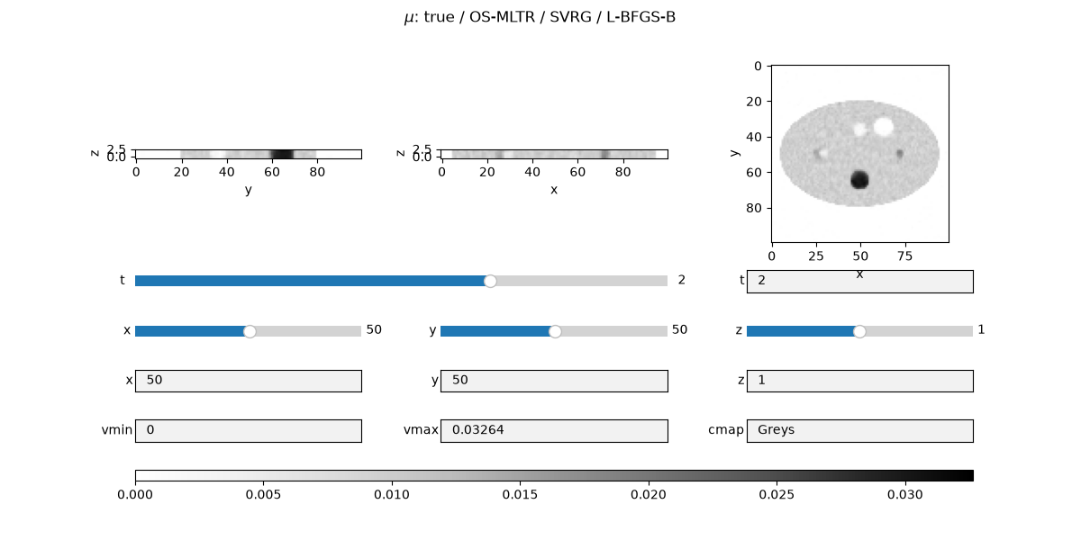
OS-MLTR and SVRG minimise the same penalised objective \(\Phi\) and reach the L-BFGS-B reference within a few epochs. The converged \(\mu\) is visibly smoother in the uniform regions while the dense inserts (edges \(\gg \delta\)) are preserved by the log-cosh penalty.

c_min = float(min(c.min() for c in cost.values()))
c_max = float(cost["SVRG"][4])

fig, ax = plt.subplots(1, 2, figsize=(11, 4.5), tight_layout=True)
for name in ("OS-MLTR", "SVRG", "L-BFGS-B"):
    ax[0].plot(cost[name], label=name)
ax[0].set_ylim(c_min, c_max)
ax[0].set_xlabel("epoch (subset methods) / function evaluation (L-BFGS-B)")
ax[0].set_ylabel(r"$\Phi(\mu) = -L(\mu) + \beta R(\mu)$")
ax[0].grid(ls=":")
ax[0].legend()

sl = img_shape[2] // 2
ax[1].plot(
    to_numpy_array(mu_true[:, img_shape[1] // 2, sl]), "k--", label=r"true $\mu$"
)
for name in ("OS-MLTR", "SVRG", "L-BFGS-B"):
    ax[1].plot(to_numpy_array(mu_final[name][:, img_shape[1] // 2, sl]), label=name)
ax[1].set_xlabel("pixel")
ax[1].set_ylabel(r"$\mu$ [1/mm]")
ax[1].grid(ls=":")
ax[1].legend()
fig.show()

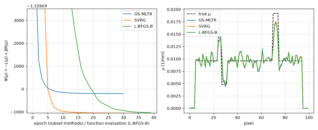
fig2 = show_vol_cuts(
    np.concatenate(
        [to_numpy_array(mu_true)[None]]
        + [to_numpy_array(mu_final[name])[None] for name in mu_final]
    ),
    voxel_size=voxel_size,
    fig_title=r"$\mu$: true / " + " / ".join(mu_final),
    vmin=0,
    vmax=3.4 * mu_water,
)

plt.show()