DePierro’s algorithm to optimize the Poisson logL with quadratic intensity prior

This example demonstrates the use of DePierro’s algorithm to minimize the negative Poisson log-likelihood function combined with a quadratic intensity prior:

\[f(x) = \sum_{i=1}^m \bar{y}_i - y_i \log(\bar{y}_i (x)) + \frac{\beta}{2} \|x - z \|^2\]

subject to

\[x \geq 0\]

using the linear forward model

\[\bar{y}(x) = A x + s\]

Tip

parallelproj is python array API compatible meaning it supports different array backends (e.g. numpy, cupy, torch, …) and devices (CPU or GPU). Choose your preferred array API xp and device dev below.

 import array_api_compat.numpy as xp

 # import array_api_compat.cupy as xp
 # import array_api_compat.torch as xp

 import parallelproj
 from array_api_compat import to_device
 import array_api_compat.numpy as np
 import matplotlib.pyplot as plt

 # choose a device (CPU or CUDA GPU)
 if "numpy" in xp.__name__:
     # using numpy, device must be cpu
     dev = "cpu"
 elif "cupy" in xp.__name__:
     # using cupy, only cuda devices are possible
     dev = xp.cuda.Device(0)
 elif "torch" in xp.__name__:
     # using torch valid choices are 'cpu' or 'cuda'
     dev = "cuda"

Setup of the forward model \(\bar{y}(x) = A x + s\)

We setup a minimal linear forward operator \(A\) respresented by a 4x4 matrix and an arbritrary contamination vector \(s\) of length 4.

Note

The OSEM implementation below works with all linear operators that subclass LinearOperator (e.g. the high-level projectors).

 # setup an arbitrary 4x4 matrix
 mat = xp.asarray(
     [
         [2.5, 1.2, 0.3, 0.1],
         [0.4, 3.1, 0.7, 0.2],
         [0.1, 0.3, 4.1, 2.5],
         [0.2, 0.5, 0.2, 0.9],
         [0.3, 0.1, 0.7, 0.2],
     ],
     dtype=xp.float64,
     device=dev,
 )

 op_A = parallelproj.MatrixOperator(mat)
 # setup an arbitrary contamination vector that has shape op_A.out_shape
 contamination = xp.asarray([0.3, 0.2, 0.1, 0.4, 0.1], dtype=xp.float64, device=dev)

Setup of ground truth and data simulation

We setup an arbitrary ground truth \(x_{true}\) and simulate noise-free and noisy data \(y\) by adding Poisson noise.

 # ground truth
 x_true = xp.asarray([5.5, 10.7, 8.2, 7.9], dtype=xp.float64, device=dev)

 # simulated noise-free data
 noise_free_data = op_A(x_true) + contamination

 # add Poisson noise
 np.random.seed(1)
 y = xp.asarray(
     np.random.poisson(parallelproj.to_numpy_array(noise_free_data)),
     device=dev,
     dtype=xp.float64,
 )

 x_prior = xp.full(op_A.in_shape, xp.min(x_true), dtype=xp.float64, device=dev)
 beta = 0.3
 num_iter = 50

 # initialize x
 x = xp.ones(op_A.in_shape, dtype=xp.float64, device=dev)

 def cost_function(x):
     exp = op_A(x) + contamination
     if (xp.min(exp) < 0) or (xp.min(x) < 0):
         res = xp.finfo(xp.float64).max
     else:
         res = (xp.sum(exp - y * xp.log(exp))) + 0.5 * beta * xp.sum((x - x_prior) ** 2)
     return res

DePierro update to minimize \(f(x)\)

We apply multiple DePierro updates

\[b = A^H 1 - \beta z\]

\[t = x A^H \frac{y}{A x + s}\]

\[x^+ = \frac{2 t}{\sqrt{b^2 + 4 \beta t} + b}\]

to calculate the minimizer of \(f(x)\) iteratively.

See [DP95] for more details.

 cost = xp.zeros(num_iter, dtype=xp.float64, device=dev)

 # "b" - modified sensitivity image
 mod_adjoint_ones = (
     op_A.adjoint(xp.ones(op_A.out_shape, dtype=xp.float64, device=dev)) - beta * x_prior
 )

 for i in range(num_iter):
     # evaluate the forward model
     exp = op_A(x) + contamination
     ratio = y / exp
     t = x * op_A.adjoint(ratio)
     x = 2 * t / (xp.sqrt(mod_adjoint_ones**2 + 4 * beta * t) + mod_adjoint_ones)
     cost[i] = cost_function(x)

 print(f"Solution after {num_iter} DePierro iterations:")
 print(x)
 print(f"cost: {cost[-1]:.6e}")

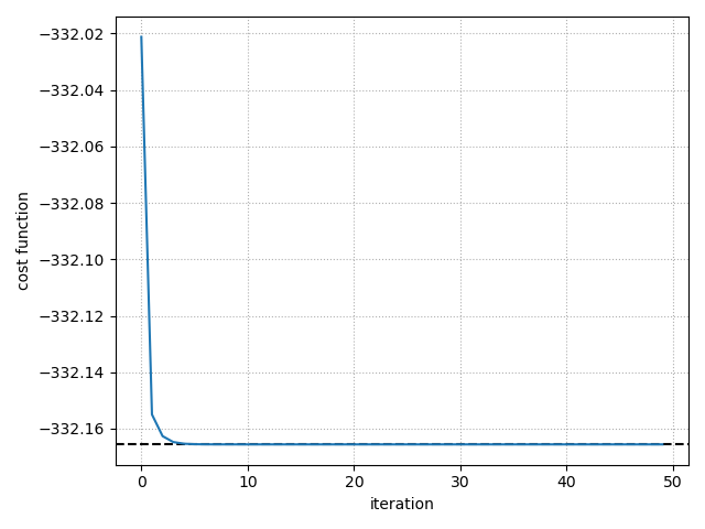
Solution after 50 DePierro iterations:
[6.28680501 7.26148792 6.72092821 6.43913514]
cost: -3.321656e+02

 if xp.__name__.endswith("numpy"):
     from scipy.optimize import fmin_powell

     x_ref = fmin_powell(cost_function, x, xtol=1e-6, ftol=1e-6)
     rel_dist = float(xp.sum((x - x_ref) ** 2)) / float(xp.sum(x_ref**2))

     print(f"\nReference solution using Powell optimizer:")
     print(x_ref)
     print(f"rel. distance to DePierro solution: {rel_dist:.2e}")
     print(f"cost: {cost_function(x_ref):.6e}")

Optimization terminated successfully.
         Current function value: -332.165557
         Iterations: 1
         Function evaluations: 113

Reference solution using Powell optimizer:
[6.28680485 7.26148793 6.72092821 6.43913496]
rel. distance to DePierro solution: 3.19e-16
cost: -3.321656e+02

 fig, ax = plt.subplots(1, 1, tight_layout=True)
 if xp.__name__.endswith("numpy"):
     ax.axhline(cost_function(x_ref), color="k", linestyle="--")
 ax.plot(parallelproj.to_numpy_array(cost))
 ax.set_xlabel("iteration")
 ax.set_ylabel("cost function")
 ax.grid(ls=":")
 fig.show()

Total running time of the script: (0 minutes 0.154 seconds)

Related examples

Basic MLEM

Basic OSEM

PDHG to optimize the Poisson logL and directional TV (structural prior)

TOF-MLEM with projection data

Gallery generated by Sphinx-Gallery