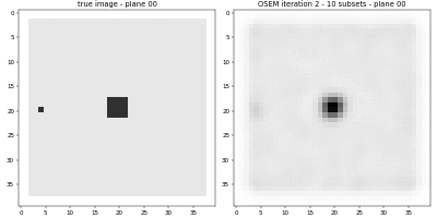
Basic OSEM

This example demonstrates the use of the MLEM algorithm with ordered subsets (OS-MLEM or OSEM) to minimize the negative Poisson log-likelihood function.

\[f(x) = \sum_{i=1}^m \bar{y}_i (x) - y_i \log(\bar{y}_i (x))\]

subject to

\[x \geq 0\]

using the linear forward model

\[\bar{y}(x) = A x + s\]

The idea is to split the complete forward operator into a sequence \(n\) disjoint subset operators

\[A = \{ A^1, \ldots, A^n \}\]

which is can be used to evaluate a subset of the forward model

\[\bar{y}^k(x) = A^k x + s^k\]

Tip

parallelproj is python array API compatible meaning it supports different array backends (e.g. numpy, cupy, torch, …) and devices (CPU or GPU). Choose your preferred array API xp and device dev below.

import array_api_compat.numpy as xp

# import array_api_compat.cupy as xp
# import array_api_compat.torch as xp

import parallelproj
from array_api_compat import to_device
import array_api_compat.numpy as np
import matplotlib.pyplot as plt

# choose a device (CPU or CUDA GPU)
if "numpy" in xp.__name__:
    # using numpy, device must be cpu
    dev = "cpu"
elif "cupy" in xp.__name__:
    # using cupy, only cuda devices are possible
    dev = xp.cuda.Device(0)
elif "torch" in xp.__name__:
    # using torch valid choices are 'cpu' or 'cuda'
    dev = "cuda"

Setup of the complete forward model \(\bar{y}(x) = A x + s\)

We setup a minimal linear forward operator \(A\) respresented by a 4x4 matrix and an arbritrary contamination vector \(s\) of length 4.

# setup an arbitrary 4x4 matrix
mat = xp.asarray(
    [
        [2.5, 1.2, 0.3, 0.1],
        [0.4, 3.1, 0.7, 0.2],
        [0.1, 0.3, 4.1, 2.5],
        [0.2, 0.5, 0.2, 0.9],
    ],
    dtype=xp.float64,
    device=dev,
)

op_A = parallelproj.MatrixOperator(mat)
# setup an arbitrary contamination vector that has shape op_A.out_shape
contamination = xp.asarray([0.3, 0.2, 0.1, 0.4], dtype=xp.float64, device=dev)

print(op_A.A)

[[2.5 1.2 0.3 0.1]
 [0.4 3.1 0.7 0.2]
 [0.1 0.3 4.1 2.5]
 [0.2 0.5 0.2 0.9]]

Setup of ground truth and data simulation

We setup an arbitrary ground truth \(x_{true}\) and simulate noise-free and noisy data \(y\) by adding Poisson noise.

# ground truth
x_true = xp.asarray([5.5, 10.7, 8.2, 7.9], dtype=xp.float64, device=dev)

# simulated noise-free data
noise_free_data = op_A(x_true) + contamination

# add Poisson noise
np.random.seed(1)
y = xp.asarray(
    np.random.poisson(parallelproj.to_numpy_array(noise_free_data)),
    device=dev,
    dtype=xp.float64,
)

Analytic calculation of the optimal point (as reference)

Since our linear forward operator \(A\) is invertible (which is usually not the case in practice), we can calculate the optimal point \(x^* = A^{-1} (y - s)\) and the corresponding optimal value of \(f(x^*)\).

# calculate the reference solution by inverting A
mat_inv = xp.linalg.inv(mat)
x_ref = mat_inv @ (y - contamination)

# also calculate the cost of the reference solution
exp_ref = op_A(x_ref) + contamination
cost_ref = float(xp.sum(exp_ref - y * xp.log(exp_ref)))

Splitting of the forward model into subsets \(A^k\)

We split the matrix operator into two disjoint subsets using slicing along the first dimension of the matrix.

Note

The OSEM implementation below works with all linear operators that subclass LinearOperatorSequence

# define two subsets (they don't need to have equal size)
subset_slices = (slice(0, 2), slice(2, None))

# setup two subsets operators each containing 1 and 3 rows of the matrix A
op_seq = parallelproj.LinearOperatorSequence(
    [parallelproj.MatrixOperator(mat[sl, :]) for sl in subset_slices]
)

for op in op_seq:
    print(op.A)

[[2.5 1.2 0.3 0.1]
 [0.4 3.1 0.7 0.2]]
[[0.1 0.3 4.1 2.5]
 [0.2 0.5 0.2 0.9]]

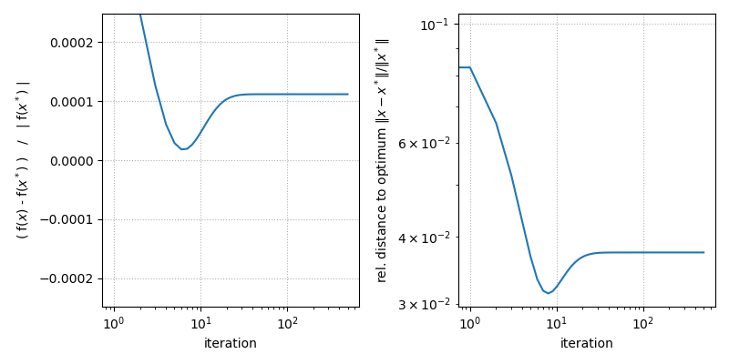
OSEM iterations to minimize \(f(x)\)

We apply multiple OSEM updates [HL94]

\[x^+ = \frac{x}{(A^k)^H 1} (A^k)^H \frac{y^k}{A^k x + s^k}\]

to calculate the minimizer of \(f(x)\) iteratively.

To monitor the convergence we calculate the relative cost

\[\frac{f(x) - f(x^*)}{|f(x^*)|}\]

and the distance to the optimal point

\[\frac{\|x - x^*\|}{\|x^*\|}.\]

# number MLEM iterations
num_iter = 1000 // len(op_seq)

# initialize x
x = xp.ones(op_A.in_shape, dtype=xp.float64, device=dev)

# calculate A_k^H 1 for all subsets k
subset_adjoint_ones = [
    x.adjoint(xp.ones(x.out_shape, dtype=xp.float64, device=dev)) for x in op_seq
]

# allocate arrays for the relative cost and the relative distance to the
# optimal point
rel_cost = xp.zeros(num_iter, dtype=xp.float64, device=dev)
rel_dist = xp.zeros(num_iter, dtype=xp.float64, device=dev)

for i in range(num_iter):
    for k, sl in enumerate(subset_slices):
        # evaluate the forward model
        subset_exp = op_seq[k](x) + contamination[sl]
        # calculate the relative cost and distance to the optimal point
        # to do this, we need the full expectation
        exp = op_A(x) + contamination
        rel_cost[i] = (xp.sum(exp - y * xp.log(exp)) - cost_ref) / abs(cost_ref)
        rel_dist[i] = xp.linalg.vector_norm(x - x_ref) / xp.linalg.vector_norm(x_ref)
        # OSEM update
        ratio = y[sl] / subset_exp
        x *= op_seq[k].adjoint(ratio) / subset_adjoint_ones[k]

Convergences plots

..note::

The basic OSEM does not converge to the optimal point (but can come close using a few number of fast updates).

fig, ax = plt.subplots(1, 2, figsize=(8, 4), sharex=True)
ax[0].semilogx(parallelproj.to_numpy_array(rel_cost))
ax[1].loglog(parallelproj.to_numpy_array(rel_dist))
ax[0].set_ylim(-rel_cost[2], rel_cost[2])
ax[0].set_ylabel(r"( f($x$) - f($x^*$) )   /   | f($x^*$) |")
ax[1].set_ylabel(r"rel. distance to optimum $\|x - x^*\| / \|x^*\|$")
ax[0].set_xlabel("iteration")
ax[1].set_xlabel("iteration")
ax[0].grid(ls=":")
ax[1].grid(ls=":")
fig.tight_layout()
fig.show()

Related examples

Basic MLEM

Basic MLEM

DePierro’s algorithm to optimize the Poisson logL with quadratic intensity prior

DePierro's algorithm to optimize the Poisson logL with quadratic intensity prior

TOF OSEM with projection data

TOF OSEM with projection data

TOF listmode OSEM with projection data

TOF listmode OSEM with projection data