MLEM with projection data of an open PET geometry

This example demonstrates the use of the MLEM algorithm to minimize the negative Poisson log-likelihood function using “sinogram” data from an open PET geometry.

\[f(x) = \sum_{i=1}^m \bar{y}_i (x) - y_i \log(\bar{y}_i (x))\]

subject to

\[x \geq 0\]

using the linear forward model

\[\bar{y}(x) = A x + s\]

Tip

parallelproj is python array API compatible meaning it supports different array backends (e.g. numpy, cupy, torch, …) and devices (CPU or GPU). Choose your preferred array API xp and device dev below.

from __future__ import annotations
from parallelproj import Array

import array_api_compat.numpy as xp

# import array_api_compat.cupy as xp
# import array_api_compat.torch as xp

import parallelproj
from array_api_compat import to_device
import array_api_compat.numpy as np
import matplotlib.pyplot as plt
import matplotlib.animation as animation

# choose a device (CPU or CUDA GPU)
if "numpy" in xp.__name__:
    # using numpy, device must be cpu
    dev = "cpu"
elif "cupy" in xp.__name__:
    # using cupy, only cuda devices are possible
    dev = xp.cuda.Device(0)
elif "torch" in xp.__name__:
    # using torch valid choices are 'cpu' or 'cuda'
    if parallelproj.cuda_present:
        dev = "cuda"
    else:
        dev = "cpu"

Setup of the forward model \(\bar{y}(x) = A x + s\)

We setup a linear forward operator \(A\) consisting of an image-based resolution model, a non-TOF PET projector and an attenuation model

Here we create an open geometry with 6 sides and 5 rings corresponding to a full geometry using 12 sides where 6 sides were removed.

num_rings = 1
scanner = parallelproj.RegularPolygonPETScannerGeometry(
    xp,
    dev,
    radius=65.0,
    num_sides=6,
    num_lor_endpoints_per_side=15,
    lor_spacing=2.3,
    ring_positions=xp.asarray([0.0], device=dev),
    symmetry_axis=2,
    phis=(2 * xp.pi / 12) * xp.asarray([-1, 0, 1, 5, 6, 7]),
)

setup the LOR descriptor that defines the sinogram

img_shape = (40, 40, 1)
voxel_size = (2.0, 2.0, 2.0)

lor_desc = parallelproj.RegularPolygonPETLORDescriptor(
    scanner,
    radial_trim=1,
    sinogram_order=parallelproj.SinogramSpatialAxisOrder.RVP,
)

proj = parallelproj.RegularPolygonPETProjector(
    lor_desc, img_shape=img_shape, voxel_size=voxel_size
)

# setup a simple test image containing a few "hot rods"
x_true = xp.ones(proj.in_shape, device=dev, dtype=xp.float32)
c0 = proj.in_shape[0] // 2
c1 = proj.in_shape[1] // 2

x_true[4, c1, :] = 5.0
x_true[8, c1, :] = 5.0
x_true[12, c1, :] = 5.0
x_true[16, c1, :] = 5.0

x_true[c0, 4, :] = 5.0
x_true[c0, 8, :] = 5.0
x_true[c0, 12, :] = 5.0
x_true[c0, 16, :] = 5.0

x_true[:2, :, :] = 0
x_true[-2:, :, :] = 0
x_true[:, :2, :] = 0
x_true[:, -2:, :] = 0

Attenuation image and sinogram setup

# setup an attenuation image
x_att = 0.01 * xp.astype(x_true > 0, xp.float32)
# calculate the attenuation sinogram
att_sino = xp.exp(-proj(x_att))

Complete PET forward model setup

We combine an image-based resolution model, a non-TOF or TOF PET projector and an attenuation model into a single linear operator.

## enable TOF - comment if you want to run non-TOF
# proj.tof_parameters = parallelproj.TOFParameters(
#    num_tofbins=13 * 5,
#    tofbin_width=12.0 / 5,
#    sigma_tof=12.0 / 5,
# )

# setup the attenuation multiplication operator which is different
# for TOF and non-TOF since the attenuation sinogram is always non-TOF
if proj.tof:
    att_op = parallelproj.TOFNonTOFElementwiseMultiplicationOperator(
        proj.out_shape, att_sino
    )
else:
    att_op = parallelproj.ElementwiseMultiplicationOperator(att_sino)

res_model = parallelproj.GaussianFilterOperator(
    proj.in_shape, sigma=4.5 / (2.35 * proj.voxel_size)
)

# compose all 3 operators into a single linear operator
pet_lin_op = parallelproj.CompositeLinearOperator((att_op, proj, res_model))

Visualization of the geometry

fig = plt.figure(figsize=(16, 8), tight_layout=True)
ax1 = fig.add_subplot(121, projection="3d")
ax2 = fig.add_subplot(122, projection="3d")
proj.show_geometry(ax1)
proj.show_geometry(ax2)
proj.lor_descriptor.show_views(
    ax1,
    views=xp.asarray([0], device=dev),
    planes=xp.asarray([num_rings // 2], device=dev),
    lw=0.5,
    color="k",
)
ax1.set_title(f"view 0, plane {num_rings // 2}")
proj.lor_descriptor.show_views(
    ax2,
    views=xp.asarray([proj.lor_descriptor.num_views // 2], device=dev),
    planes=xp.asarray([num_rings // 2], device=dev),
    lw=0.5,
    color="k",
)
ax2.set_title(f"view {proj.lor_descriptor.num_views // 2}, plane {num_rings // 2}")
fig.tight_layout()
fig.show()

Simulation of projection data

We setup an arbitrary ground truth \(x_{true}\) and simulate noise-free and noisy data \(y\) by adding Poisson noise.

# simulated noise-free data
noise_free_data = pet_lin_op(x_true)

# generate a contant contamination sinogram
contamination = xp.full(
    noise_free_data.shape,
    0.5 * float(xp.mean(noise_free_data)),
    device=dev,
    dtype=xp.float32,
)

noise_free_data += contamination

# add Poisson noise
# np.random.seed(1)
# y = xp.asarray(
#    np.random.poisson(parallelproj.to_numpy_array(noise_free_data)),
#    device=dev,
#    dtype=xp.float64,
# )

y = noise_free_data

EM update to minimize \(f(x)\)

The EM update that can be used in MLEM or OSEM is given by cite:p:Dempster1977 [SV82] [LC84] [HL94]

\[x^+ = \frac{x}{(A^k)^H 1} (A^k)^H \frac{y^k}{A^k x + s^k}\]

to calculate the minimizer of \(f(x)\) iteratively.

To monitor the convergence we calculate the relative cost

\[\frac{f(x) - f(x^*)}{|f(x^*)|}\]

and the distance to the optimal point

\[\frac{\|x - x^*\|}{\|x^*\|}.\]

We setup a function that calculates a single MLEM/OSEM update given the current solution, a linear forward operator, data, contamination and the adjoint of ones.

def em_update(
    x_cur: Array,
    data: Array,
    op: parallelproj.LinearOperator,
    s: Array,
    adjoint_ones: Array,
) -> Array:
    """EM update

    Parameters
    ----------
    x_cur : Array
        current solution
    data : Array
        data
    op : parallelproj.LinearOperator
        linear forward operator
    s : Array
        contamination
    adjoint_ones : Array
        adjoint of ones

    Returns
    -------
    Array
        _description_
    """
    ybar = op(x_cur) + s
    return x_cur * op.adjoint(data / ybar) / adjoint_ones

Run the MLEM iterations

# number of MLEM iterations
num_iter = 100

# initialize x
x = xp.ones(pet_lin_op.in_shape, dtype=xp.float32, device=dev)
# calculate A^H 1
adjoint_ones = pet_lin_op.adjoint(
    xp.ones(pet_lin_op.out_shape, dtype=xp.float32, device=dev)
)

for i in range(num_iter):
    print(f"MLEM iteration {(i + 1):03} / {num_iter:03}", end="\r")
    x = em_update(x, y, pet_lin_op, contamination, adjoint_ones)

MLEM iteration 001 / 100
MLEM iteration 002 / 100
MLEM iteration 003 / 100
MLEM iteration 004 / 100
MLEM iteration 005 / 100
MLEM iteration 006 / 100
MLEM iteration 007 / 100
MLEM iteration 008 / 100
MLEM iteration 009 / 100
MLEM iteration 010 / 100
MLEM iteration 011 / 100
MLEM iteration 012 / 100
MLEM iteration 013 / 100
MLEM iteration 014 / 100
MLEM iteration 015 / 100
MLEM iteration 016 / 100
MLEM iteration 017 / 100
MLEM iteration 018 / 100
MLEM iteration 019 / 100
MLEM iteration 020 / 100
MLEM iteration 021 / 100
MLEM iteration 022 / 100
MLEM iteration 023 / 100
MLEM iteration 024 / 100
MLEM iteration 025 / 100
MLEM iteration 026 / 100
MLEM iteration 027 / 100
MLEM iteration 028 / 100
MLEM iteration 029 / 100
MLEM iteration 030 / 100
MLEM iteration 031 / 100
MLEM iteration 032 / 100
MLEM iteration 033 / 100
MLEM iteration 034 / 100
MLEM iteration 035 / 100
MLEM iteration 036 / 100
MLEM iteration 037 / 100
MLEM iteration 038 / 100
MLEM iteration 039 / 100
MLEM iteration 040 / 100
MLEM iteration 041 / 100
MLEM iteration 042 / 100
MLEM iteration 043 / 100
MLEM iteration 044 / 100
MLEM iteration 045 / 100
MLEM iteration 046 / 100
MLEM iteration 047 / 100
MLEM iteration 048 / 100
MLEM iteration 049 / 100
MLEM iteration 050 / 100
MLEM iteration 051 / 100
MLEM iteration 052 / 100
MLEM iteration 053 / 100
MLEM iteration 054 / 100
MLEM iteration 055 / 100
MLEM iteration 056 / 100
MLEM iteration 057 / 100
MLEM iteration 058 / 100
MLEM iteration 059 / 100
MLEM iteration 060 / 100
MLEM iteration 061 / 100
MLEM iteration 062 / 100
MLEM iteration 063 / 100
MLEM iteration 064 / 100
MLEM iteration 065 / 100
MLEM iteration 066 / 100
MLEM iteration 067 / 100
MLEM iteration 068 / 100
MLEM iteration 069 / 100
MLEM iteration 070 / 100
MLEM iteration 071 / 100
MLEM iteration 072 / 100
MLEM iteration 073 / 100
MLEM iteration 074 / 100
MLEM iteration 075 / 100
MLEM iteration 076 / 100
MLEM iteration 077 / 100
MLEM iteration 078 / 100
MLEM iteration 079 / 100
MLEM iteration 080 / 100
MLEM iteration 081 / 100
MLEM iteration 082 / 100
MLEM iteration 083 / 100
MLEM iteration 084 / 100
MLEM iteration 085 / 100
MLEM iteration 086 / 100
MLEM iteration 087 / 100
MLEM iteration 088 / 100
MLEM iteration 089 / 100
MLEM iteration 090 / 100
MLEM iteration 091 / 100
MLEM iteration 092 / 100
MLEM iteration 093 / 100
MLEM iteration 094 / 100
MLEM iteration 095 / 100
MLEM iteration 096 / 100
MLEM iteration 097 / 100
MLEM iteration 098 / 100
MLEM iteration 099 / 100
MLEM iteration 100 / 100

Calculation of the negative Poisson log-likelihood function of the reconstruction

# calculate the negative Poisson log-likelihood function of the reconstruction
exp = pet_lin_op(x) + contamination
# calculate the relative cost and distance to the optimal point
cost = float(xp.sum(exp - y * xp.log(exp)))
print(f"\nMLEM cost {cost:.6E} after {num_iter:03} iterations")

MLEM cost -2.586407E+05 after 100 iterations

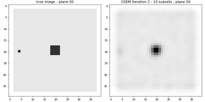
Visualize the results

def _update_img(i):
    img0.set_data(x_true_np[:, :, i])
    img1.set_data(x_np[:, :, i])
    ax[0].set_title(f"true image - plane {i:02}")
    ax[1].set_title(f"MLEM iteration {num_iter} - plane {i:02}")
    return (img0, img1)


x_true_np = parallelproj.to_numpy_array(x_true)
x_np = parallelproj.to_numpy_array(x)

fig, ax = plt.subplots(1, 2, figsize=(10, 5))
vmax = x_np.max()
img0 = ax[0].imshow(x_true_np[:, :, 0], cmap="Greys", vmin=0, vmax=vmax)
img1 = ax[1].imshow(x_np[:, :, 0], cmap="Greys", vmin=0, vmax=vmax)
ax[0].set_title(f"true image - plane {0:02}")
ax[1].set_title(f"MLEM iteration {num_iter} - plane {0:02}")
fig.tight_layout()
ani = animation.FuncAnimation(fig, _update_img, x_np.shape[2], interval=200, blit=False)
fig.show()

Once Loop Reflect

Related examples

TOF-MLEM with projection data

TOF-MLEM with projection data

TOF listmode MLEM with projection data

TOF listmode MLEM with projection data

TOF OSEM with projection data

TOF OSEM with projection data

TOF listmode OSEM with projection data

TOF listmode OSEM with projection data