Non-TOF and TOF projections using a modularized (block) PET scanner geometry

In this example, we show how to perform non-TOF and TOF projections using a PET scanner consisting of multiple block modules where each block module consists of a regular grid of LOR endpoints.

import math
import matplotlib.pyplot as plt
from vis import show_vol_cuts

import parallelproj.pet_scanners
import parallelproj.pet_lors
import parallelproj.projectors
import parallelproj.tof
from parallelproj import to_numpy_array

from array_utils import suggest_array_backend_and_device

# To use a specific backend and/or device, replace the None arguments, e.g.:
#   xp, dev = suggest_array_backend_and_device(backend="numpy", dev="cpu") or by setting xp and dev manually
xp, dev = suggest_array_backend_and_device(None, None)

Using array API: array_api_compat.torch, device: cpu

input paraters

# grid shape of LOR endpoints forming a block module
block_shape = (3, 2, 2)
# spacing between LOR endpoints in a block module
block_spacing = (1.5, 1.2, 1.7)
# radius of the scanner
scanner_radius = 10

Setup of a modularized PET scanner geometry

We define 7 block modules arranged in a circle with a radius of 10. The arangement follows a regular polygon with 12 sides, leaving some of the sides empty. Note that all block modules must be identical, but can be anywhere in space. The location of a block module can be changed using an affine transformation matrix.

mods = []

delta_phi = 2 * xp.pi / 12

# setup an affine transformation matrix to translate the block modules from the
# center to the radius of the scanner
aff_mat_trans = xp.eye(4, device=dev)
aff_mat_trans[1, -1] = scanner_radius

for phi in [
    -delta_phi,
    0,
    delta_phi,
    5 * delta_phi,
    6 * delta_phi,
    7 * delta_phi,
]:
    # setup an affine transformation matrix to rotate the block modules around the center
    # (of the "2" axis)
    aff_mat_rot = xp.asarray(
        [
            [math.cos(phi), -math.sin(phi), 0, 0],
            [math.sin(phi), math.cos(phi), 0, 0],
            [0, 0, 1, 0],
            [0, 0, 0, 1],
        ],
        device=dev,
    )
    mods.append(
        parallelproj.pet_scanners.BlockPETScannerModule(
            xp,
            dev,
            block_shape,
            block_spacing,
            affine_transformation_matrix=(aff_mat_rot @ aff_mat_trans),
        )
    )

# create the scanner geometry from a list of identical block modules at
# different locations in space
scanner = parallelproj.pet_scanners.ModularizedPETScannerGeometry(mods)

Setup of a LOR descriptor consisting of block pairs

Once the geometry of the LOR endpoints is defined, we can define the LORs by specifying which block pairs are in coincidence and for “valid” LORs. To do this, we have manually define a list containing pairs of block numbers. Here, we define 9 block pairs. Note that more pairs would be possible.

lor_desc = parallelproj.pet_lors.EqualBlockPETLORDescriptor(
    scanner,
    xp.asarray(
        [
            [0, 3],
            [0, 4],
            [0, 5],
            [1, 3],
            [1, 4],
            [1, 5],
            [2, 3],
            [2, 4],
            [2, 5],
        ]
    ),
)

Setup of a non-TOF projector

Now that the LOR descriptor is defined, we can setup the projector.

img_shape = (28, 20, 3)
voxel_size = (0.5, 0.5, 1.0)
img = xp.ones(img_shape, dtype=xp.float32, device=dev)

proj = parallelproj.projectors.EqualBlockPETProjector(lor_desc, img_shape, voxel_size)
assert proj.adjointness_test(xp, dev, dtype=xp.float32)

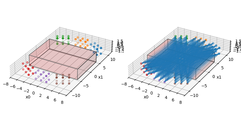
Visualize the projector geometry and all LORs

fig = plt.figure(figsize=(8, 4), tight_layout=True)
ax0 = fig.add_subplot(121, projection="3d")
ax1 = fig.add_subplot(122, projection="3d")
proj.show_geometry(ax0)
proj.show_geometry(ax1)
lor_desc.show_block_pair_lors(ax1, block_pair_nums=None, color=plt.cm.tab10(0))
fig.show()

Forward project an image full of ones. The forward projection has the shape (num_block_pairs, num_lors_per_block_pair)

img_fwd = proj(img)
print(img_fwd.shape)

torch.Size([9, 144])

Backproject a “histogram” full of ones (“sensitivity image” when attenuation and normalization are ignored)

ones_back = proj.adjoint(xp.ones(proj.out_shape, dtype=xp.float32, device=dev))
print(ones_back.shape)

torch.Size([28, 20, 3])

Visualize the forward and backward projection results

fig3, ax3 = plt.subplots(figsize=(8, 2), tight_layout=True)
ax3.imshow(to_numpy_array(img_fwd), cmap="Greys", aspect=3.0)
ax3.set_xlabel("LOR number in block pair")
ax3.set_ylabel("block pair")
ax3.set_title("forward projection of ones")
fig3.show()

fig4, _, widgets4 = show_vol_cuts(
    to_numpy_array(ones_back), fig_title="back projection of ones"
)
fig4.show()

• 
• 

Setup of a TOF projector

Now that the LOR descriptor is defined, we can setup the projector.

proj_tof = parallelproj.projectors.EqualBlockPETProjector(
    lor_desc, img_shape, voxel_size
)
proj_tof.tof_parameters = parallelproj.tof.TOFParameters(
    num_tofbins=27, tofbin_width=0.8, sigma_tof=2.0, num_sigmas=3.0
)

assert proj_tof.adjointness_test(xp, dev, dtype=xp.float32)

TOF forward project an image full of ones. The forward projection has the shape (num_block_pairs, num_lors_per_block_pair, num_tofbins)

img_fwd_tof = proj_tof(img)
print(img_fwd_tof.shape)

torch.Size([9, 144, 27])

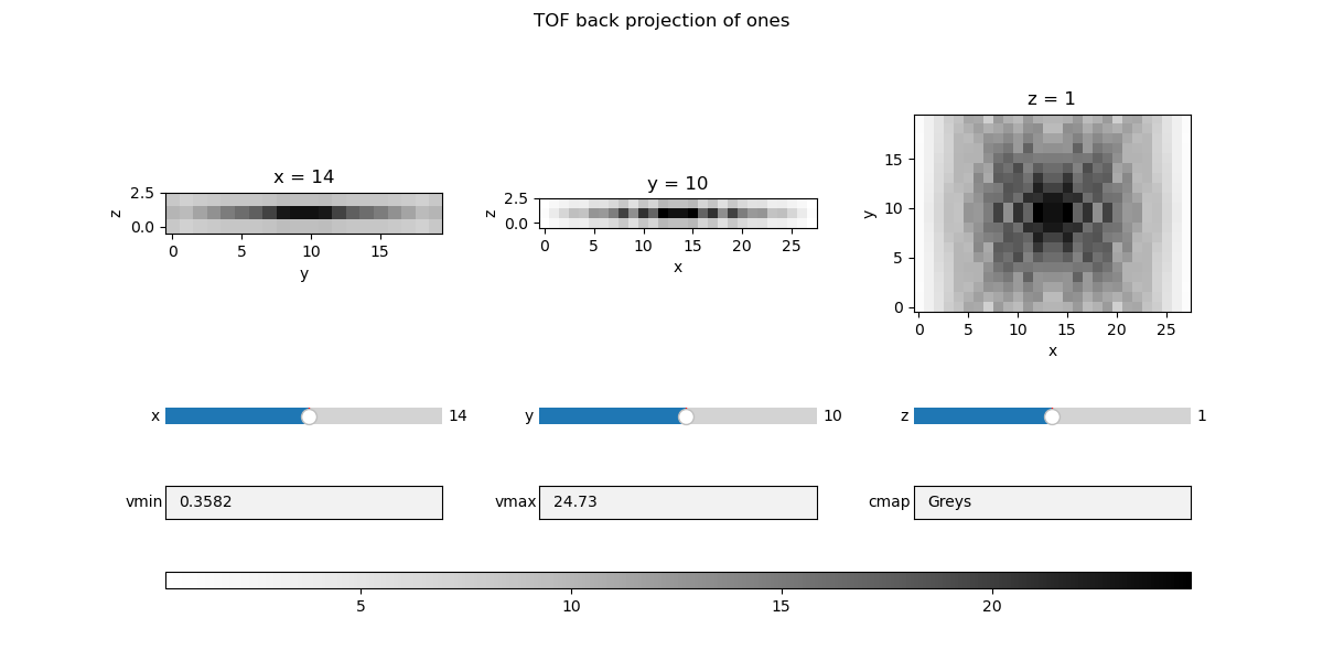
TOF backproject a “TOF histogram” full of ones (“sensitivity image” when attenuation and normalization are ignored)

ones_back_tof = proj_tof.adjoint(
    xp.ones(proj_tof.out_shape, dtype=xp.float32, device=dev)
)
print(ones_back_tof.shape)

torch.Size([28, 20, 3])

Visualize the forward and backward projection results

fig5, ax5 = plt.subplots(figsize=(6, 3), tight_layout=True)
ax5.plot(to_numpy_array(img_fwd_tof[0, 0, :]), ".-")
ax5.set_xlabel("TOF bin")
ax5.set_title("TOF profile of LOR 0 in block pair 0")
fig5.show()

fig6, _, widgets6 = show_vol_cuts(
    to_numpy_array(ones_back_tof), fig_title="TOF back projection of ones"
)
fig6.show()