DePierro’s algorithm to optimize the Poisson logL with quadratic intensity prior

This example demonstrates the use of DePierro’s algorithm to minimize the negative Poisson log-likelihood function combined with a quadratic intensity prior:

\[f(x) = \sum_{i=1}^m \bar{y}_i - y_i \log(\bar{y}_i (x)) + \frac{\beta}{2} \|x - z \|^2\]

subject to

\[x \geq 0\]

using the linear forward model

\[\bar{y}(x) = A x + s\]

import matplotlib.pyplot as plt
import numpy as np

import parallelproj.operators
from parallelproj import to_numpy_array

from array_utils import suggest_array_backend_and_device

# To use a specific backend and/or device, replace the None arguments, e.g.:
#   xp, dev = suggest_array_backend_and_device(backend="numpy", dev="cpu") or by setting xp and dev manually
xp, dev = suggest_array_backend_and_device(None, None)

Using array API: array_api_compat.torch, device: cpu

Setup of the forward model \(\bar{y}(x) = A x + s\)

We setup a minimal linear forward operator \(A\) respresented by a 4x4 matrix and an arbritrary contamination vector \(s\) of length 4.

Note

The OSEM implementation below works with all linear operators that subclass LinearOperator (e.g. the high-level projectors).

# setup an arbitrary 4x4 matrix
mat = xp.asarray(
    [
        [2.5, 1.2, 0.3, 0.1],
        [0.4, 3.1, 0.7, 0.2],
        [0.1, 0.3, 4.1, 2.5],
        [0.2, 0.5, 0.2, 0.9],
        [0.3, 0.1, 0.7, 0.2],
    ],
    dtype=xp.float64,
    device=dev,
)

op_A = parallelproj.operators.MatrixOperator(mat)
# setup an arbitrary contamination vector that has shape op_A.out_shape
contamination = xp.asarray([0.3, 0.2, 0.1, 0.4, 0.1], dtype=xp.float64, device=dev)

Setup of ground truth and data simulation

We setup an arbitrary ground truth \(x_{true}\) and simulate noise-free and noisy data \(y\) by adding Poisson noise.

# ground truth
x_true = xp.asarray([5.5, 10.7, 8.2, 7.9], dtype=xp.float64, device=dev)

# simulated noise-free data
noise_free_data = op_A(x_true) + contamination

# add Poisson noise
np.random.seed(1)
y = xp.asarray(
    np.random.poisson(to_numpy_array(noise_free_data)),
    device=dev,
    dtype=xp.float64,
)

x_prior = xp.full(op_A.in_shape, xp.min(x_true), dtype=xp.float64, device=dev)
beta = 0.3
num_iter = 50

# initialize x
x = xp.ones(op_A.in_shape, dtype=xp.float64, device=dev)

def cost_function(x):
    exp = op_A(x) + contamination
    if (xp.min(exp) < 0) or (xp.min(x) < 0):
        res = xp.finfo(xp.float64).max
    else:
        res = (xp.sum(exp - y * xp.log(exp))) + 0.5 * beta * xp.sum((x - x_prior) ** 2)
    return res

DePierro update to minimize \(f(x)\)

We apply multiple DePierro updates

\[b = A^H 1 - \beta z\]

\[t = x A^H \frac{y}{A x + s}\]

\[x^+ = \frac{2 t}{\sqrt{b^2 + 4 \beta t} + b}\]

to calculate the minimizer of \(f(x)\) iteratively.

See [DP95] for more details.

cost = xp.zeros(num_iter, dtype=xp.float64, device=dev)

# "b" - modified sensitivity image
mod_adjoint_ones = (
    op_A.adjoint(xp.ones(op_A.out_shape, dtype=xp.float64, device=dev)) - beta * x_prior
)

for i in range(num_iter):
    # evaluate the forward model
    exp = op_A(x) + contamination
    ratio = y / exp
    t = x * op_A.adjoint(ratio)
    x = 2 * t / (xp.sqrt(mod_adjoint_ones**2 + 4 * beta * t) + mod_adjoint_ones)
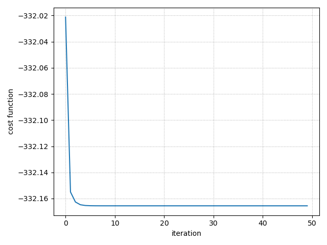
    cost[i] = cost_function(x)

print(f"Solution after {num_iter} DePierro iterations:")
print(x)
print(f"cost: {cost[-1]:.6e}")

Solution after 50 DePierro iterations:
tensor([6.2868, 7.2615, 6.7209, 6.4391], dtype=torch.float64)
cost: -3.321656e+02

if xp.__name__.endswith("numpy"):
    from scipy.optimize import fmin_powell

    x_ref = fmin_powell(cost_function, x, xtol=1e-6, ftol=1e-6)
    rel_dist = float(xp.sum((x - x_ref) ** 2)) / float(xp.sum(x_ref**2))

    print(f"\nReference solution using Powell optimizer:")
    print(x_ref)
    print(f"rel. distance to DePierro solution: {rel_dist:.2e}")
    print(f"cost: {cost_function(x_ref):.6e}")

fig, ax = plt.subplots(1, 1, tight_layout=True)
if xp.__name__.endswith("numpy"):
    ax.axhline(cost_function(x_ref), color="k", linestyle="--")
ax.plot(to_numpy_array(cost))
ax.set_xlabel("iteration")
ax.set_ylabel("cost function")
ax.grid(ls=":")
fig.show()