Functions `parallelproj.functions`¶

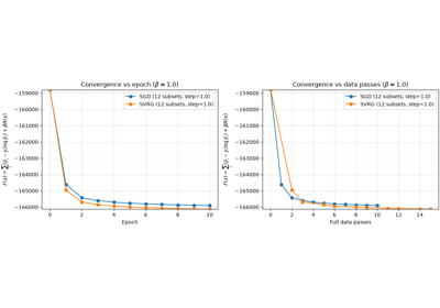
Convergence comparison: SGD vs SVRG with logcosh regularization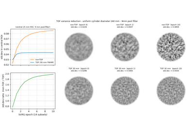

TOF vs non-TOF: variance reduction in a uniform cylinder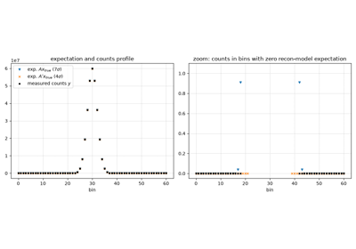

Exact vs. “safe epsilon” mode of the negative Poisson log-likelihood

Exact vs. "safe epsilon" mode of the negative Poisson log-likelihood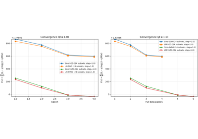

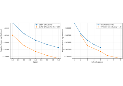
Convergence comparison: SGD vs SVRG with regularization (sinogram and listmode)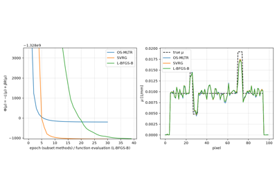

Penalised transmission reconstruction (MAPTR) with an edge-preserving prior

__call__(x: Array) → float¶

Evaluate \(\beta f(x)\).

Parameters:: x (Array) – Point at which to evaluate the function.
Returns:: Scaled scalar function value.
Return type:: float

Examples

property beta: float¶: Multiplicative scale factor \(\beta\) (should be > 0).

call_and_gradient(x: Array) → tuple[float, Array]¶

Evaluate \(\beta f(x)\) and its gradient simultaneously.

Parameters:: x (Array) – Point at which to evaluate.
Returns:: Scaled function value and gradient.
Return type:: tuple[float, Array]

Examples

gradient(x: Array) → Array¶

Gradient of \(\beta f(x)\).

Parameters:: x (Array) – Point at which to evaluate the gradient.
Returns:: Array of the same shape as x containing \(\beta \nabla f(x)\).
Return type:: Array

Examples

Exact vs. “safe epsilon” mode of the negative Poisson log-likelihood

Exact vs. "safe epsilon" mode of the negative Poisson log-likelihood

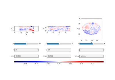
Penalised transmission reconstruction (MAPTR) with an edge-preserving prior

class parallelproj.functions.C1Function(beta: float = 1.0)[source]¶

Bases: ABC

Abstract base class for continuously differentiable (C1) scalar functions with an optional scalar scale factor \(\beta\).

The public interface (__call__(), gradient(), call_and_gradient()) evaluates \(\beta f(x)\). Subclasses only implement the unscaled private methods _call() and _gradient(); \(\beta\) is applied automatically.

Parameters:: beta (float, optional) – Multiplicative scale factor \(\beta\) applied to the function value and all derivatives. Defaults to 1.0.

Examples

Convergence comparison: SGD vs SVRG with logcosh regularization

PDHG and SPDHG for PET reconstruction with a directional TV prior

TOF vs non-TOF: variance reduction in a uniform cylinder

Exact vs. “safe epsilon” mode of the negative Poisson log-likelihood

Exact vs. "safe epsilon" mode of the negative Poisson log-likelihood

Convergence comparison: SGD vs SVRG with regularization (sinogram and listmode)

Penalised transmission reconstruction (MAPTR) with an edge-preserving prior

__call__(x: Array) → float[source]¶

Evaluate \(\beta f(x)\).

Parameters:: x (Array) – Point at which to evaluate the function.
Returns:: Scaled scalar function value.
Return type:: float

Examples

property beta: float¶: Multiplicative scale factor \(\beta\) (should be > 0).

call_and_gradient(x: Array) → tuple[float, Array][source]¶

Evaluate \(\beta f(x)\) and its gradient simultaneously.

Parameters:: x (Array) – Point at which to evaluate.
Returns:: Scaled function value and gradient.
Return type:: tuple[float, Array]

Examples

gradient(x: Array) → Array[source]¶

Gradient of \(\beta f(x)\).

Parameters:: x (Array) – Point at which to evaluate the gradient.
Returns:: Array of the same shape as x containing \(\beta \nabla f(x)\).
Return type:: Array

Examples

Exact vs. “safe epsilon” mode of the negative Poisson log-likelihood

Exact vs. "safe epsilon" mode of the negative Poisson log-likelihood

Penalised transmission reconstruction (MAPTR) with an edge-preserving prior

class parallelproj.functions.C1FunctionWithConjProx(beta: float = 1.0)[source]¶

Bases: C1Function, FunctionWithConjProx

Abstract base class for C1 functions that also admit a closed-form proximal operator of their convex conjugate.

Use this as the base class when your function is differentiable and has a cheap closed-form \(\operatorname{prox}_{\sigma f^*}\). Subclasses must implement _call(), _gradient(), and _prox_convex_conj(). The \(\beta\) scaling and the public prox_convex_conj() wrapper are inherited and require no override.

See NegPoissonLogL and HalfSquaredL2Deviation for concrete examples.

Examples

Convergence comparison: SGD vs SVRG with logcosh regularization

PDHG and SPDHG for PET reconstruction with a directional TV prior

TOF vs non-TOF: variance reduction in a uniform cylinder

Exact vs. “safe epsilon” mode of the negative Poisson log-likelihood

Exact vs. "safe epsilon" mode of the negative Poisson log-likelihood

Convergence comparison: SGD vs SVRG with regularization (sinogram and listmode)

Parameters:: beta (float)

__call__(x: Array) → float¶

Evaluate \(\beta f(x)\).

Parameters:: x (Array) – Point at which to evaluate the function.
Returns:: Scaled scalar function value.
Return type:: float

Examples

property beta: float¶: Multiplicative scale factor \(\beta\) (should be > 0).

call_and_gradient(x: Array) → tuple[float, Array]¶

Evaluate \(\beta f(x)\) and its gradient simultaneously.

Parameters:: x (Array) – Point at which to evaluate.
Returns:: Scaled function value and gradient.
Return type:: tuple[float, Array]

Examples

gradient(x: Array) → Array¶

Gradient of \(\beta f(x)\).

Parameters:: x (Array) – Point at which to evaluate the gradient.
Returns:: Array of the same shape as x containing \(\beta \nabla f(x)\).
Return type:: Array

Examples

Exact vs. “safe epsilon” mode of the negative Poisson log-likelihood

Exact vs. "safe epsilon" mode of the negative Poisson log-likelihood

prox(x: Array, sigma: float | Array) → Array¶

Proximal operator of \(\beta f\) via Moreau’s identity.

\[\text{prox}_{\sigma (\beta f)}(x) = x - \sigma \, \text{prox}_{(1/\sigma)(\beta f)^*}(x / \sigma)\]

where the inner prox uses step-size \(1/\sigma\).

Subclasses with a cheaper closed-form direct prox may override this.

Parameters:

x (Array) – Input array.
sigma (float or Array) – Step-size parameter \(\sigma > 0\).

Returns:

\(\text{prox}_{\sigma (\beta f)}(x)\).

Return type:

Array

Examples

prox_convex_conj(y: Array, sigma: float | Array) → Array¶

Proximal operator of the convex conjugate of \(\beta f\).

Uses the identity

\[\text{prox}_{\sigma (\beta f)^*}(y) = \beta \, \text{prox}_{(\sigma / \beta)\, f^*}(y / \beta)\]

to reduce to the unscaled _prox_convex_conj().

Parameters:

y (Array) – Input array.
sigma (float or Array) – Step-size parameter \(\sigma > 0\).

Returns:

\(\text{prox}_{\sigma (\beta f)^*}(y)\).

Return type:

Array

Examples

class parallelproj.functions.C2AffineObjective(loss: C2Function, op: LinearOperator, s: Array | None = None)[source]¶

Bases: C2Function, C1AffineObjective

Composes a prediction-space C2Function with an affine forward model.

Extends C1AffineObjective with second-order information. For \(f(x) = g(A x + s)\) the Hessian-vector product is:

\[H_f(x)\, v = A^H \bigl(\operatorname{diag}(H_g(\bar{y})) \odot (A v)\bigr)\]

where \(\bar{y} = A x + s\) (or \(\bar{y} = A x\) when \(s\) is None) and \(\odot\) denotes elementwise multiplication. Any scaling is carried exclusively by the beta attribute of loss.

Parameters:

loss (C2Function) – A C2Function operating on the prediction space.
op (LinearOperator) – The linear part of the forward model \(A\).
s (Array or None, optional) – Additive contamination term \(s\) (e.g. scatter/randoms). None (default) selects the pure linear model \(\bar{y} = A x\).

Examples

>>> import numpy as np
>>> from parallelproj.operators import MatrixOperator
>>> from parallelproj.functions import NegPoissonLogL, C2AffineObjective
>>> # 4-element image space, 6-element sinogram space
>>> A = np.random.rand(6, 4)
>>> op = MatrixOperator(A)
>>> s = 0.1 * np.ones(6)          # scatter/randoms contamination
>>> data = np.ones(6)             # measured counts
>>> x = np.ones(4)                # image estimate
>>> v = np.ones(4)                # direction vector
>>>
>>> loss = NegPoissonLogL(data)
>>> loss.beta = 0.5
>>> aff_obj = C2AffineObjective(loss, op, s)
>>>
>>> fx = aff_obj(x)                           # scalar value, scaled by beta=0.5
>>> grad = aff_obj.gradient(x)                          # shape (4,), scaled by beta=0.5
>>> hv   = aff_obj.hessian_diag_vec_prod(x, v)          # shape (4,), scaled by beta=0.5

Pure linear forward model with virtual bins (zero rows in \(A\)), handled by NegPoissonLogL – the default (“safe epsilon”) mode is finite everywhere; exact=True would also work here since the virtual bins measure 0:

>>> A2 = np.zeros((6, 4))
>>> A2[:4, :] = np.random.rand(4, 4)   # last 2 rows are virtual (all zero)
>>> op2   = MatrixOperator(A2)
>>> data2 = np.array([2., 1., 3., 0., 0., 0.])  # virtual bins measure 0
>>>
>>> loss2 = NegPoissonLogL(data2)
>>> aff_obj2 = C2AffineObjective(loss2, op2)            # no contamination s
>>>
>>> fx2   = aff_obj2(x)                                 # scalar function value, no nan
>>> grad2 = aff_obj2.gradient(x)                        # shape (4,), no nan
>>> hv2   = aff_obj2.hessian_diag_vec_prod(x, v)        # shape (4,), no nan

A regularised objective combining a data fidelity term and a roughness penalty via SumC2Function:

\[h(x) = \underbrace{f_{\text{PL}}(Ax + s)}_{\text{data fidelity}} + \underbrace{\beta_{\text{reg}} \cdot \tfrac{1}{2}\|Dx\|_2^2}_{\text{roughness penalty}}\]

where \(D\) is a finite forward difference operator.

>>> from parallelproj.operators import FiniteForwardDifference
>>> from parallelproj.functions import HalfSquaredL2Deviation
>>> beta_reg = 0.1
>>> D   = FiniteForwardDifference(x.shape)            # finite differences in image space
>>> reg = C2AffineObjective(HalfSquaredL2Deviation(beta=beta_reg), D)
>>> data_fidelity = C2AffineObjective(NegPoissonLogL(data), op, s)
>>>
>>> obj_fun = data_fidelity + reg                     # SumC2Function
>>> obj_val = obj_fun(x)                              # scalar function value
>>> grad = obj_fun.gradient(x)                        # shape (4,)
>>> hv   = obj_fun.hessian_diag_vec_prod(x, v)        # shape (4,)

Examples

Convergence comparison: SGD vs SVRG with logcosh regularization

TOF vs non-TOF: variance reduction in a uniform cylinder

Exact vs. “safe epsilon” mode of the negative Poisson log-likelihood

Exact vs. "safe epsilon" mode of the negative Poisson log-likelihood

Convergence comparison: SGD vs SVRG with regularization (sinogram and listmode)

Penalised transmission reconstruction (MAPTR) with an edge-preserving prior

Joint activity and attenuation reconstruction (MLAA) for TOF PET

__call__(x: Array) → float¶

Evaluate \(\beta f(x)\).

Parameters:: x (Array) – Point at which to evaluate the function.
Returns:: Scaled scalar function value.
Return type:: float

Examples

property beta: float¶: Multiplicative scale factor \(\beta\) (should be > 0).

call_and_gradient(x: Array) → tuple[float, Array]¶

Evaluate \(\beta f(x)\) and its gradient simultaneously.

Parameters:: x (Array) – Point at which to evaluate.
Returns:: Scaled function value and gradient.
Return type:: tuple[float, Array]

Examples

gradient(x: Array) → Array¶

Gradient of \(\beta f(x)\).

Parameters:: x (Array) – Point at which to evaluate the gradient.
Returns:: Array of the same shape as x containing \(\beta \nabla f(x)\).
Return type:: Array

Examples

Exact vs. “safe epsilon” mode of the negative Poisson log-likelihood

Exact vs. "safe epsilon" mode of the negative Poisson log-likelihood

Penalised transmission reconstruction (MAPTR) with an edge-preserving prior

hessian_diag_vec_prod(x: Array, v: Array) → Array¶

Scaled diagonal Hessian-vector product: \(\beta \operatorname{diag}(H_f(x))\, v\).

Parameters:

x (Array) – Point at which to evaluate the Hessian diagonal.
v (Array) – Vector to multiply with the Hessian diagonal, same shape as x.

Returns:

Array of the same shape as x containing \(\beta \operatorname{diag}(H_f(x)) \odot v\) (elementwise).

Return type:

Array

Examples

Convergence comparison: SGD vs SVRG with logcosh regularization

Convergence comparison: SGD vs SVRG with regularization (sinogram and listmode)

class parallelproj.functions.C2Function(beta: float = 1.0)[source]¶

Bases: C1Function

Abstract base class for twice continuously differentiable (C2) scalar functions with an optional scalar scale factor \(\beta\).

Extends C1Function with curvature information. The public hessian_diag_vec_prod() returns \(\beta \operatorname{diag}(H_f(x))\, v\). Subclasses implement the unscaled _hessian_diag_vec_prod().

Examples

Convergence comparison: SGD vs SVRG with logcosh regularization

PDHG and SPDHG for PET reconstruction with a directional TV prior

TOF vs non-TOF: variance reduction in a uniform cylinder

Exact vs. “safe epsilon” mode of the negative Poisson log-likelihood

Exact vs. "safe epsilon" mode of the negative Poisson log-likelihood

Convergence comparison: SGD vs SVRG with regularization (sinogram and listmode)

Penalised transmission reconstruction (MAPTR) with an edge-preserving prior

Parameters:: beta (float)

__call__(x: Array) → float¶

Evaluate \(\beta f(x)\).

Parameters:: x (Array) – Point at which to evaluate the function.
Returns:: Scaled scalar function value.
Return type:: float

Examples

property beta: float¶: Multiplicative scale factor \(\beta\) (should be > 0).

call_and_gradient(x: Array) → tuple[float, Array]¶

Evaluate \(\beta f(x)\) and its gradient simultaneously.

Parameters:: x (Array) – Point at which to evaluate.
Returns:: Scaled function value and gradient.
Return type:: tuple[float, Array]

Examples

gradient(x: Array) → Array¶

Gradient of \(\beta f(x)\).

Parameters:: x (Array) – Point at which to evaluate the gradient.
Returns:: Array of the same shape as x containing \(\beta \nabla f(x)\).
Return type:: Array

Examples

Exact vs. “safe epsilon” mode of the negative Poisson log-likelihood

Exact vs. "safe epsilon" mode of the negative Poisson log-likelihood

Penalised transmission reconstruction (MAPTR) with an edge-preserving prior

hessian_diag_vec_prod(x: Array, v: Array) → Array[source]¶

Scaled diagonal Hessian-vector product: \(\beta \operatorname{diag}(H_f(x))\, v\).

Parameters:

x (Array) – Point at which to evaluate the Hessian diagonal.
v (Array) – Vector to multiply with the Hessian diagonal, same shape as x.

Returns:

Array of the same shape as x containing \(\beta \operatorname{diag}(H_f(x)) \odot v\) (elementwise).

Return type:

Array

Examples

Convergence comparison: SGD vs SVRG with logcosh regularization

Convergence comparison: SGD vs SVRG with regularization (sinogram and listmode)

class parallelproj.functions.C2FunctionWithConjProx(beta: float = 1.0)[source]¶

Bases: C2Function, C1FunctionWithConjProx

Abstract base class for C2 functions that also admit a closed-form proximal operator of their convex conjugate.

Combines C2Function (Hessian diagonal) with C1FunctionWithConjProx (gradient, call, dual prox). Subclasses must implement _call(), _gradient(), _hessian_diag_vec_prod(), and _prox_convex_conj().

MRO: C2FunctionWithConjProx -> C2Function -> C1FunctionWithConjProx -> C1Function -> FunctionWithConjProx -> ABC

Examples

Convergence comparison: SGD vs SVRG with logcosh regularization

PDHG and SPDHG for PET reconstruction with a directional TV prior

TOF vs non-TOF: variance reduction in a uniform cylinder

Exact vs. “safe epsilon” mode of the negative Poisson log-likelihood

Exact vs. "safe epsilon" mode of the negative Poisson log-likelihood

Convergence comparison: SGD vs SVRG with regularization (sinogram and listmode)

Parameters:: beta (float)

__call__(x: Array) → float¶

Evaluate \(\beta f(x)\).

Parameters:: x (Array) – Point at which to evaluate the function.
Returns:: Scaled scalar function value.
Return type:: float

Examples

property beta: float¶: Multiplicative scale factor \(\beta\) (should be > 0).

call_and_gradient(x: Array) → tuple[float, Array]¶

Evaluate \(\beta f(x)\) and its gradient simultaneously.

Parameters:: x (Array) – Point at which to evaluate.
Returns:: Scaled function value and gradient.
Return type:: tuple[float, Array]

Examples

gradient(x: Array) → Array¶

Gradient of \(\beta f(x)\).

Parameters:: x (Array) – Point at which to evaluate the gradient.
Returns:: Array of the same shape as x containing \(\beta \nabla f(x)\).
Return type:: Array

Examples

Exact vs. “safe epsilon” mode of the negative Poisson log-likelihood

Exact vs. "safe epsilon" mode of the negative Poisson log-likelihood

hessian_diag_vec_prod(x: Array, v: Array) → Array¶

Scaled diagonal Hessian-vector product: \(\beta \operatorname{diag}(H_f(x))\, v\).

Parameters:

x (Array) – Point at which to evaluate the Hessian diagonal.
v (Array) – Vector to multiply with the Hessian diagonal, same shape as x.

Returns:

Array of the same shape as x containing \(\beta \operatorname{diag}(H_f(x)) \odot v\) (elementwise).

Return type:

Array

Examples

prox(x: Array, sigma: float | Array) → Array¶

Proximal operator of \(\beta f\) via Moreau’s identity.

\[\text{prox}_{\sigma (\beta f)}(x) = x - \sigma \, \text{prox}_{(1/\sigma)(\beta f)^*}(x / \sigma)\]

where the inner prox uses step-size \(1/\sigma\).

Subclasses with a cheaper closed-form direct prox may override this.

Parameters:

x (Array) – Input array.
sigma (float or Array) – Step-size parameter \(\sigma > 0\).

Returns:

\(\text{prox}_{\sigma (\beta f)}(x)\).

Return type:

Array

Examples

prox_convex_conj(y: Array, sigma: float | Array) → Array¶

Proximal operator of the convex conjugate of \(\beta f\).

Uses the identity

\[\text{prox}_{\sigma (\beta f)^*}(y) = \beta \, \text{prox}_{(\sigma / \beta)\, f^*}(y / \beta)\]

to reduce to the unscaled _prox_convex_conj().

Parameters:

y (Array) – Input array.
sigma (float or Array) – Step-size parameter \(\sigma > 0\).

Returns:

\(\text{prox}_{\sigma (\beta f)^*}(y)\).

Return type:

Array

Examples

class parallelproj.functions.FunctionWithConjProx(beta: float = 1.0)[source]¶

Bases: ABC

Abstract base class for functions with a closed-form proximal operator of their convex conjugate.

This class is a standalone root – it does not require the function to be differentiable. Non-smooth functions (e.g. total variation, indicator functions) that admit a closed-form \(\text{prox}_{\sigma f^*}\) should inherit directly from this class.

Differentiable functions that additionally have a closed-form dual prox should use C1FunctionWithConjProx or C2FunctionWithConjProx instead.

The public prox_convex_conj() handles the \(\beta\) scaling automatically. Subclasses implement only the unscaled private methods _call() and _prox_convex_conj().

A default prox() is provided via Moreau’s identity for convenience; subclasses may override it with a more efficient closed-form if available.

Parameters:: beta (float, optional) – Multiplicative scale factor \(\beta\). Defaults to 1.0.

Examples

Convergence comparison: SGD vs SVRG with logcosh regularization

PDHG and SPDHG for PET reconstruction with a directional TV prior

TOF vs non-TOF: variance reduction in a uniform cylinder

Exact vs. “safe epsilon” mode of the negative Poisson log-likelihood

Exact vs. "safe epsilon" mode of the negative Poisson log-likelihood

Convergence comparison: SGD vs SVRG with regularization (sinogram and listmode)

__call__(x: Array) → float[source]¶

Evaluate \(\beta f(x)\).

Parameters:: x (Array) – Point at which to evaluate the function.
Returns:: Scaled scalar function value \(\beta f(x)\).
Return type:: float

Examples

property beta: float¶: Multiplicative scale factor \(\beta\) (should be > 0).

prox(x: Array, sigma: float | Array) → Array[source]¶

Proximal operator of \(\beta f\) via Moreau’s identity.

\[\text{prox}_{\sigma (\beta f)}(x) = x - \sigma \, \text{prox}_{(1/\sigma)(\beta f)^*}(x / \sigma)\]

where the inner prox uses step-size \(1/\sigma\).

Subclasses with a cheaper closed-form direct prox may override this.

Parameters:

x (Array) – Input array.
sigma (float or Array) – Step-size parameter \(\sigma > 0\).

Returns:

\(\text{prox}_{\sigma (\beta f)}(x)\).

Return type:

Array

Examples

prox_convex_conj(y: Array, sigma: float | Array) → Array[source]¶

Proximal operator of the convex conjugate of \(\beta f\).

Uses the identity

\[\text{prox}_{\sigma (\beta f)^*}(y) = \beta \, \text{prox}_{(\sigma / \beta)\, f^*}(y / \beta)\]

to reduce to the unscaled _prox_convex_conj().

Parameters:

y (Array) – Input array.
sigma (float or Array) – Step-size parameter \(\sigma > 0\).

Returns:

\(\text{prox}_{\sigma (\beta f)^*}(y)\).

Return type:

Array

Examples

class parallelproj.functions.FunctionWithProx(beta: float = 1.0)[source]¶

Bases: ABC

Abstract base class for functions with a closed-form proximal operator.

This class is a standalone root – it does not require the function to be differentiable. Functions (e.g. indicator functions, L1 norm) that admit a closed-form \(\text{prox}_{\sigma f}\) should inherit directly from this class.

The public prox() handles the \(\beta\) scaling automatically. Subclasses implement only the unscaled private methods _call() and _prox().

A default prox_convex_conj() is provided via Moreau’s identity for convenience; subclasses may override it with a more efficient closed-form if available.

Parameters:: beta (float, optional) – Multiplicative scale factor \(\beta\). Defaults to 1.0.

Examples

PDHG and SPDHG for PET reconstruction with a directional TV prior

__call__(x: Array) → float[source]¶

Evaluate \(\beta f(x)\).

Parameters:: x (Array) – Point at which to evaluate the function.
Returns:: Scaled scalar function value \(\beta f(x)\).
Return type:: float

Examples

property beta: float¶: Multiplicative scale factor \(\beta\) (should be > 0).

prox(x: Array, sigma: float | Array) → Array[source]¶

Proximal operator of \(\beta f\).

\[\text{prox}_{\sigma (\beta f)}(x) = \text{prox}_{(\sigma \beta) f}(x)\]

so the effective step size passed to the unscaled _prox() is \(\sigma \beta\).

Parameters:

x (Array) – Input array.
sigma (float or Array) – Step-size parameter \(\sigma > 0\).

Returns:

\(\text{prox}_{\sigma (\beta f)}(x)\).

Return type:

Array

Examples

prox_convex_conj(y: Array, sigma: float | Array) → Array[source]¶

Proximal operator of the convex conjugate of \(\beta f\) via Moreau’s identity.

\[\text{prox}_{\sigma (\beta f)^*}(y) = y - \sigma \, \text{prox}_{(1/\sigma)(\beta f)}(y / \sigma)\]

where the inner prox uses step-size \(1/\sigma\).

Subclasses with a cheaper closed-form dual prox may override this.

Parameters:

y (Array) – Input array.
sigma (float or Array) – Step-size parameter \(\sigma > 0\).

Returns:

\(\text{prox}_{\sigma (\beta f)^*}(y)\).

Return type:

Array

Examples

class parallelproj.functions.HalfSquaredL2Deviation(data: Array | None = None, weights: Array | None = None, beta: float = 1.0)[source]¶

Bases: C2FunctionWithConjProx

Half squared L2 deviation from reference data, with optional weights.

Implements

\[f(x) = \frac{1}{2} \sum_i w_i (x_i - d_i)^2\]

where \(w_i = 1\) when no weights are supplied (reducing to the standard \(\tfrac{1}{2}\|x - d\|_2^2\)).

Gradient:

\[\nabla f(x) = w \odot (x - d)\]

Diagonal Hessian-vector product:

\[\operatorname{diag}(H_f(x)) \odot v = w \odot v\]

The \(\tfrac{1}{2}\) prefactor is chosen so that the gradient contains no factor of 2, keeping expressions clean when \(\beta = 1\).

Parameters:

data (Array or None, optional) – Reference array \(d\). None (default) is equivalent to \(d = 0\) but avoids the subtraction entirely.
weights (Array or None, optional) – Non-negative weight array \(w\) of the same shape as data (or x when data is None). None (default) is equivalent to unit weights but avoids the multiplication entirely.
beta (float, optional) – Multiplicative scale factor \(\beta\). Defaults to 1.0.

Examples

__call__(x: Array) → float¶

Evaluate \(\beta f(x)\).

Parameters:: x (Array) – Point at which to evaluate the function.
Returns:: Scaled scalar function value.
Return type:: float

Examples

property beta: float¶: Multiplicative scale factor \(\beta\) (should be > 0).

call_and_gradient(x: Array) → tuple[float, Array]¶

Evaluate \(\beta f(x)\) and its gradient simultaneously.

Parameters:: x (Array) – Point at which to evaluate.
Returns:: Scaled function value and gradient.
Return type:: tuple[float, Array]

Examples

gradient(x: Array) → Array¶

Gradient of \(\beta f(x)\).

Parameters:: x (Array) – Point at which to evaluate the gradient.
Returns:: Array of the same shape as x containing \(\beta \nabla f(x)\).
Return type:: Array

Examples

hessian_diag_vec_prod(x: Array, v: Array) → Array¶

Scaled diagonal Hessian-vector product: \(\beta \operatorname{diag}(H_f(x))\, v\).

Parameters:

x (Array) – Point at which to evaluate the Hessian diagonal.
v (Array) – Vector to multiply with the Hessian diagonal, same shape as x.

Returns:

Array of the same shape as x containing \(\beta \operatorname{diag}(H_f(x)) \odot v\) (elementwise).

Return type:

Array

Examples

prox(x: Array, sigma: float | Array) → Array¶

Proximal operator of \(\beta f\) via Moreau’s identity.

\[\text{prox}_{\sigma (\beta f)}(x) = x - \sigma \, \text{prox}_{(1/\sigma)(\beta f)^*}(x / \sigma)\]

where the inner prox uses step-size \(1/\sigma\).

Subclasses with a cheaper closed-form direct prox may override this.

Parameters:

x (Array) – Input array.
sigma (float or Array) – Step-size parameter \(\sigma > 0\).

Returns:

\(\text{prox}_{\sigma (\beta f)}(x)\).

Return type:

Array

Examples

prox_convex_conj(y: Array, sigma: float | Array) → Array¶

Proximal operator of the convex conjugate of \(\beta f\).

Uses the identity

\[\text{prox}_{\sigma (\beta f)^*}(y) = \beta \, \text{prox}_{(\sigma / \beta)\, f^*}(y / \beta)\]

to reduce to the unscaled _prox_convex_conj().

Parameters:

y (Array) – Input array.
sigma (float or Array) – Step-size parameter \(\sigma > 0\).

Returns:

\(\text{prox}_{\sigma (\beta f)^*}(y)\).

Return type:

Array

Examples

class parallelproj.functions.LogCosh(delta: float | None = None, beta: float = 1.0)[source]¶

Bases: C2Function

Sum of scaled log-cosh values, a smooth approximation to the L1 norm.

Implements

\[f(x) = \delta \sum_i \log\!\left(\cosh\!\left(\frac{x_i}{\delta}\right)\right)\]

where \(\delta > 0\) is a transition scale parameter (default 1). The function satisfies \(f(0) = 0\) and has two limiting regimes:

Quadratic for \(|x_i| \ll \delta\): \(\delta\log(\cosh(u)) \approx u^2/2\), so \(f(x) \approx \tfrac{1}{2\delta}\sum_i x_i^2\).
Linear for \(|x_i| \gg \delta\): \(f(x) \approx \sum_i |x_i| - n\,\delta\log 2 \approx \sum_i |x_i|\).

The \(\delta\) prefactor ensures the asymptotic slope equals 1 regardless of \(\delta\), so the transition scale and the gradient magnitude at saturation are decoupled.

Gradient:

\[\nabla f(x)_i = \tanh\!\left(\frac{x_i}{\delta}\right)\]

Diagonal Hessian-vector product:

\[\operatorname{diag}(H_f(x))_i \cdot v_i = \frac{1}{\delta}\,\operatorname{sech}^2\!\left(\frac{x_i}{\delta}\right) v_i = \frac{1 - \tanh^2(x_i/\delta)}{\delta}\, v_i\]

The function value is computed via the numerically stable identity

\[\delta\log(\cosh(z)) = \delta\bigl(|z| + \log(1 + e^{-2|z|}) - \log 2\bigr), \quad z = x/\delta\]

which avoids the overflow that \(\cosh(z) = (e^z + e^{-z})/2\) would cause for large \(|z|\).

Parameters:

delta (float or None, optional) – Transition scale \(\delta > 0\). None (default) is equivalent to \(\delta = 1\) but skips the division entirely.
beta (float, optional) – Multiplicative scale factor \(\beta\). Defaults to 1.0.

Notes

The function value computation uses math.prod(x.shape) to subtract the normalisation constant \(n \log 2\). This requires that x.shape is a concrete tuple of integers at call time, which holds for all supported backends (NumPy, CuPy, PyTorch) but would fail for frameworks with symbolic or lazy shapes.

Examples

Convergence comparison: SGD vs SVRG with logcosh regularization

Convergence comparison: SGD vs SVRG with regularization (sinogram and listmode)

Penalised transmission reconstruction (MAPTR) with an edge-preserving prior

Joint activity and attenuation reconstruction (MLAA) for TOF PET

__call__(x: Array) → float¶

Evaluate \(\beta f(x)\).

Parameters:: x (Array) – Point at which to evaluate the function.
Returns:: Scaled scalar function value.
Return type:: float

Examples

property beta: float¶: Multiplicative scale factor \(\beta\) (should be > 0).

call_and_gradient(x: Array) → tuple[float, Array]¶

Evaluate \(\beta f(x)\) and its gradient simultaneously.

Parameters:: x (Array) – Point at which to evaluate.
Returns:: Scaled function value and gradient.
Return type:: tuple[float, Array]

Examples

property delta: float | None¶: Transition scale \(\delta\).

gradient(x: Array) → Array¶

Gradient of \(\beta f(x)\).

Parameters:: x (Array) – Point at which to evaluate the gradient.
Returns:: Array of the same shape as x containing \(\beta \nabla f(x)\).
Return type:: Array

Examples

hessian_diag_vec_prod(x: Array, v: Array) → Array¶

Scaled diagonal Hessian-vector product: \(\beta \operatorname{diag}(H_f(x))\, v\).

Parameters:

x (Array) – Point at which to evaluate the Hessian diagonal.
v (Array) – Vector to multiply with the Hessian diagonal, same shape as x.

Returns:

Array of the same shape as x containing \(\beta \operatorname{diag}(H_f(x)) \odot v\) (elementwise).

Return type:

Array

Examples

class parallelproj.functions.MixedL21Norm(beta: float = 1.0)[source]¶

Bases: FunctionWithConjProx

Mixed L2-L1 norm (isotropic TV semi-norm on a gradient field).

For an array \(g\) whose first axis enumerates the gradient directions (as produced by FiniteForwardDifference), the norm is

\[f(g) = \sum_{\mathbf{i}} \|g_{:, \mathbf{i}}\|_2\]

where the sum runs over all spatial multi-indices \(\mathbf{i}\) and the L2 norm is taken along axis 0.

The convex conjugate is the indicator of the mixed \(L_{\infty,2}\) unit ball:

\[\begin{split}f^*(p) = \begin{cases} 0 & \|p_{:, \mathbf{i}}\|_2 \leq 1 \; \forall \mathbf{i} \\ +\infty & \text{otherwise} \end{cases}\end{split}\]

so its proximal operator is a pointwise projection onto the L2 unit ball along axis 0 (independent of \(\sigma\)):

\[\left(\text{prox}_{\sigma f^*}(y)\right)_{:, \mathbf{i}} = \frac{y_{:, \mathbf{i}}}{\max\!\left(\|y_{:, \mathbf{i}}\|_2,\, 1\right)}\]

The direct prox() (block soft-thresholding) is available via Moreau’s identity.

Parameters:: beta (float, optional) – Multiplicative scale factor \(\beta\) (regularization weight). Defaults to 1.0.

Examples

PDHG and SPDHG for PET reconstruction with a directional TV prior

__call__(x: Array) → float¶

Evaluate \(\beta f(x)\).

Parameters:: x (Array) – Point at which to evaluate the function.
Returns:: Scaled scalar function value \(\beta f(x)\).
Return type:: float

Examples

property beta: float¶: Multiplicative scale factor \(\beta\) (should be > 0).

prox(x: Array, sigma: float | Array) → Array¶

Proximal operator of \(\beta f\) via Moreau’s identity.

\[\text{prox}_{\sigma (\beta f)}(x) = x - \sigma \, \text{prox}_{(1/\sigma)(\beta f)^*}(x / \sigma)\]

where the inner prox uses step-size \(1/\sigma\).

Subclasses with a cheaper closed-form direct prox may override this.

Parameters:

x (Array) – Input array.
sigma (float or Array) – Step-size parameter \(\sigma > 0\).

Returns:

\(\text{prox}_{\sigma (\beta f)}(x)\).

Return type:

Array

Examples

prox_convex_conj(y: Array, sigma: float | Array) → Array¶

Proximal operator of the convex conjugate of \(\beta f\).

Uses the identity

\[\text{prox}_{\sigma (\beta f)^*}(y) = \beta \, \text{prox}_{(\sigma / \beta)\, f^*}(y / \beta)\]

to reduce to the unscaled _prox_convex_conj().

Parameters:

y (Array) – Input array.
sigma (float or Array) – Step-size parameter \(\sigma > 0\).

Returns:

\(\text{prox}_{\sigma (\beta f)^*}(y)\).

Return type:

Array

Examples

class parallelproj.functions.NegPoissonLogL(data: Array, beta: float = 1.0, exact: bool = False, rel_eps: float = 1e-06, eps: float | None = None, enable_extra_checks: bool = False)[source]¶

Bases: C2FunctionWithConjProx

Negative Poisson log-likelihood as a function of expected counts.

Implements

\[f(\bar{y}) = \sum_i \bar{y}_i - y_i \log \bar{y}_i\]

and its gradient w.r.t. the expected counts \(\bar{y}\):

\[\nabla_{\bar{y}} f = 1 - \frac{y}{\bar{y}}.\]

This class operates directly on the predicted counts \(\bar{y}\) (passed as the argument x to the callable interface), independently of how they were computed. Use C2AffineObjective to compose with a forward model \(\bar{y}(x) = A x + s\).

Evaluation modes

exact=False (default, “safe epsilon” mode)

All methods evaluate the shifted Poisson surrogate

\[f_\varepsilon(\bar{y}) = \sum_i (\bar{y}_i + \varepsilon) - (y_i + \varepsilon) \log(\bar{y}_i + \varepsilon)\]

i.e. exactly the Poisson log-likelihood of the shifted data evaluated at the shifted expectation, with gradient \((\bar{y} - y)/(\bar{y} + \varepsilon)\) and Hessian diagonal \((y + \varepsilon)/(\bar{y} + \varepsilon)^2\), corresponding to a tiny known contamination \(\varepsilon\) added to both the data and the expectation. It is smooth and finite for all \(\bar{y} \geq 0\) (never nan / inf), and the per-bin minimiser remains exactly at \(\bar{y}_i = y_i\): the gradient error w.r.t. the unshifted log-likelihood is \(\varepsilon (y - \bar{y}) / (\bar{y} (\bar{y} + \varepsilon))\), proportional to the residual and vanishing at the fit. By default \(\varepsilon\) = rel_eps * mean(y).

exact=True

The unmodified log-likelihood. Bins with \(y_i = 0\) (virtual bins without geometric sensitivity, and active bins that measured zero counts) are handled exactly via their analytic values (\(f_i = \bar{y}_i\), gradient \(1\), Hessian diagonal \(0\)), so this mode requires only \(\bar{y}_i > 0\) in bins with \(y_i > 0\) – guaranteed e.g. by a strictly positive contamination in all non-virtual bins. If that requirement is violated, the value is \(+\infty\) and the gradient \(-\infty\) (mathematically correct: counts were observed where the model predicts none; numpy emits a RuntimeWarning, cupy and torch produce the infinities silently).

Use exact=True whenever \(\bar{y}_i = 0\) can be ruled out in every bin with counts; otherwise keep the default.

Note

Prox-driven algorithms (PDHG / SPDHG) never divide by \(\bar{y}\) – the closed-form dual prox is stable even for zero-count bins – so with a strictly positive contamination they should use exact=True and solve the exact problem. In the default mode, prox_convex_conj() is shifted consistently so that all methods of an instance refer to the same (surrogate) objective.

Choosing eps. The default rel_eps = 1e-6 is appropriate for float32 data in units of counts (mean counts per bin roughly between 0.01 and 1000, covering TOF and non-TOF PET): the bias stays orders of magnitude below Poisson noise while \((y+\varepsilon)/ \varepsilon^2\) stays far from float32 overflow. When several instances must sum exactly to a full objective (subset algorithms), derive one global eps = rel_eps * float(xp.mean(y_full)) and pass it explicitly to every instance – otherwise each subset derives a slightly different \(\varepsilon\) from its own data mean.

Parameters:

data (Array) – Measured data \(y\) (non-negative).
beta (float, optional) – Multiplicative scale factor \(\beta\). Defaults to 1.0.
exact (bool, optional) – If True, evaluate the unmodified log-likelihood (with exact handling of bins where \(y_i = 0\)). Requires \(\bar{y}_i > 0\) in every bin with \(y_i > 0\). Defaults to False (shifted-Poisson surrogate, always finite).
rel_eps (float, optional) – Relative epsilon used to derive \(\varepsilon\) = rel_eps * mean(y) in the default mode. Ignored when exact=True or when eps is given. Defaults to 1e-6.
eps (float, optional) – Absolute \(\varepsilon\) override (must be > 0). Useful to share one global epsilon across subset objectives. Ignored when exact=True.
enable_extra_checks (bool, optional) – If True, inspect x on every evaluation of the function value, gradient, or Hessian-diagonal product and emit a RuntimeWarning for problematic inputs (negative values; in exact mode also non-positive values at bins with counts, which yield \(\pm\infty\)). Useful for debugging with cupy / torch, which – unlike numpy – produce nan / inf silently. The checks cost one reduction and a device-to-host sync per call, so they are off by default.

Examples

Convergence comparison: SGD vs SVRG with logcosh regularization

PDHG and SPDHG for PET reconstruction with a directional TV prior

TOF vs non-TOF: variance reduction in a uniform cylinder

Exact vs. “safe epsilon” mode of the negative Poisson log-likelihood

Exact vs. "safe epsilon" mode of the negative Poisson log-likelihood

Convergence comparison: SGD vs SVRG with regularization (sinogram and listmode)

__call__(x: Array) → float¶

Evaluate \(\beta f(x)\).

Parameters:: x (Array) – Point at which to evaluate the function.
Returns:: Scaled scalar function value.
Return type:: float

Examples

property beta: float¶: Multiplicative scale factor \(\beta\) (should be > 0).

call_and_gradient(x: Array) → tuple[float, Array]¶

Evaluate \(\beta f(x)\) and its gradient simultaneously.

Parameters:: x (Array) – Point at which to evaluate.
Returns:: Scaled function value and gradient.
Return type:: tuple[float, Array]

Examples

property enable_extra_checks: bool¶: Whether input checks (with warnings) are performed on every evaluation.

property eps: float¶: Effective epsilon of the shifted-Poisson surrogate (0.0 in exact mode).

property exact: bool¶: Whether the unmodified (exact) log-likelihood is evaluated.

gradient(x: Array) → Array¶

Gradient of \(\beta f(x)\).

Parameters:: x (Array) – Point at which to evaluate the gradient.
Returns:: Array of the same shape as x containing \(\beta \nabla f(x)\).
Return type:: Array

Examples

Exact vs. “safe epsilon” mode of the negative Poisson log-likelihood

Exact vs. "safe epsilon" mode of the negative Poisson log-likelihood

hessian_diag_vec_prod(x: Array, v: Array) → Array¶

Scaled diagonal Hessian-vector product: \(\beta \operatorname{diag}(H_f(x))\, v\).

Parameters:

x (Array) – Point at which to evaluate the Hessian diagonal.
v (Array) – Vector to multiply with the Hessian diagonal, same shape as x.

Returns:

Array of the same shape as x containing \(\beta \operatorname{diag}(H_f(x)) \odot v\) (elementwise).

Return type:

Array

Examples

prox(x: Array, sigma: float | Array) → Array¶

Proximal operator of \(\beta f\) via Moreau’s identity.

\[\text{prox}_{\sigma (\beta f)}(x) = x - \sigma \, \text{prox}_{(1/\sigma)(\beta f)^*}(x / \sigma)\]

where the inner prox uses step-size \(1/\sigma\).

Subclasses with a cheaper closed-form direct prox may override this.

Parameters:

x (Array) – Input array.
sigma (float or Array) – Step-size parameter \(\sigma > 0\).

Returns:

\(\text{prox}_{\sigma (\beta f)}(x)\).

Return type:

Array

Examples

prox_convex_conj(y: Array, sigma: float | Array) → Array¶

Proximal operator of the convex conjugate of \(\beta f\).

Uses the identity

\[\text{prox}_{\sigma (\beta f)^*}(y) = \beta \, \text{prox}_{(\sigma / \beta)\, f^*}(y / \beta)\]

to reduce to the unscaled _prox_convex_conj().

Parameters:

y (Array) – Input array.
sigma (float or Array) – Step-size parameter \(\sigma > 0\).

Returns:

\(\text{prox}_{\sigma (\beta f)^*}(y)\).

Return type:

Array

Examples

class parallelproj.functions.NegPoissonLogLListmode(lm_op: LinearOperator, sensitivity_image: Array, contamination_list: Array, contamination_sinogram_sum: float, eps: float = 0.0)[source]¶

Bases: C2Function

Negative Poisson log-likelihood for listmode (event-by-event) data.

Implements the listmode equivalent of NegPoissonLogL with an affine forward model \(\bar{y}_e = (A_{\text{LM}}\, x)_e + s_e\). The function value is

\[f(x) = \langle \text{sens},\, x \rangle + c_{\text{sino}} - \sum_{e=1}^{N_{\text{ev}}} \log\bigl((A_{\text{LM}}\,x)_e + s_e\bigr)\]

where

\(\text{sens} = A_{\text{full}}^T \mathbf{1}\) is the sensitivity image (backprojection of all-ones from the full sinogram),
\(c_{\text{sino}} = \sum_i s_i^{\text{sino}}\) is the scalar sum of the contamination over all sinogram bins, and
the sum runs over all \(N_{\text{ev}}\) detected events.

This is mathematically equivalent to the sinogram NegPoissonLogL because \(\sum_e \log \bar{y}_{j_e} = \sum_i y_i \log \bar{y}_i\) (each event from bin \(i\) contributes \(\log \bar{y}_i\) and there are \(y_i\) such events).

The gradient with respect to the image \(x\) is

\[\nabla_x f(x) = \text{sens} - A_{\text{LM}}^T \!\left(\frac{1}{A_{\text{LM}}\,x + s_{\text{LM}}}\right)\]

and the diagonal Hessian-vector product is

\[\operatorname{diag}(H_f(x)) \odot v = A_{\text{LM}}^T \!\left( \frac{A_{\text{LM}}\, v}{(A_{\text{LM}}\,x + s_{\text{LM}})^2} \right).\]

Note

Unlike NegPoissonLogL, the forward model \(A_{\text{LM}}\) is built into this class rather than being supplied externally. Wrapping it with C2AffineObjective would double-compose the forward model and is therefore not supported.

Note

No analogue of the safe handling of NegPoissonLogL is needed here: bins with \(y_i = 0\) cannot appear in the event list, so the indeterminate \(0 \cdot \log 0\) / \(0/0\) cases are excluded by construction. The only remaining failure mode is a detected event with zero predicted counts (\(\bar{y}_e = 0\), equivalent to \(y_i > 0\), \(\bar{y}_i = 0\) in sinogram space), which is a genuine model violation. With the default eps = 0, every call to __call__(), gradient(), or hessian_diag_vec_prod() therefore requires that all per-event predicted counts \((A_{\text{LM}}\,x)_e + s_e\) are strictly positive – guaranteed by a strictly positive contamination_list, which is the normal situation in practice. A ValueError is raised otherwise.

Optional epsilon smoothing (eps > 0). When a strictly positive per-event contamination cannot be guaranteed (e.g. no contamination and a truncated / mismatched forward model), setting eps > 0 evaluates the smoothed objective

\[f_\varepsilon(x) = \langle \text{sens},\, x \rangle + c_{\text{sino}} - \sum_e \log\bigl(\bar{y}_e + \varepsilon\bigr),\]

which in sinogram space equals \(\sum_i \bar{y}_i - y_i \log(\bar{y}_i + \varepsilon)\) – the epsilon shift applied to the expectation only. This is finite for all \(\bar{y}_e \geq 0\) and self-consistent (value, gradient, and Hessian derive from one convex function).

Note

The shifted Poisson surrogate of NegPoissonLogL (epsilon added to the data and the expectation) cannot be implemented in listmode: its data-shift term \(\varepsilon \sum_i \log(\bar{y}_i + \varepsilon)\) sums over all sinogram bins and would require a full sinogram forward/backprojection per evaluation, defeating the purpose of listmode processing. As a consequence, the expectation-only shift used here has its per-bin minimiser at \(\bar{y}_i = y_i - \varepsilon\) (a bias of \(-\varepsilon\), negligible for small \(\varepsilon\) since event bins have \(y_i \geq 1\)), and the listmode and sinogram objectives differ at \(O(\varepsilon)\) when both use their epsilon modes.

A good choice is eps = 1e-6 * n_events / num_data_bins (i.e. \(10^{-6}\) times the mean emission sinogram value), with n_events = contamination_list.shape[0] and num_data_bins taken from the projector / LOR descriptor of the full forward model used to compute the sensitivity image (e.g. math.prod(proj.out_shape)).

Parameters:

lm_op (LinearOperator) – Listmode forward projector \(A_{\text{LM}}\) mapping an image (shape: n_voxels) to per-event predicted counts (shape: n_events).
sensitivity_image (Array) – Sensitivity image \(A_{\text{full}}^T \mathbf{1}\) (same shape as the image \(x\)).
contamination_list (Array) – Per-event additive contamination \(s_{\text{LM}}\) (same shape as the listmode output, i.e. n_events).
contamination_sinogram_sum (float) – Scalar sum of the contamination over all sinogram bins, \(c_{\text{sino}} = \sum_i s_i^{\text{sino}}\).
eps (float, optional) – Epsilon added to the per-event predicted counts in all log / division terms (see above). Defaults to 0.0 (exact log-likelihood), assuming a strictly positive contamination for every event.

Examples

Convergence comparison: SGD vs SVRG with regularization (sinogram and listmode)

__call__(x: Array) → float¶

Evaluate \(\beta f(x)\).

Parameters:: x (Array) – Point at which to evaluate the function.
Returns:: Scaled scalar function value.
Return type:: float

Examples

property beta: float¶: Multiplicative scale factor \(\beta\) (should be > 0).

call_and_gradient(x: Array) → tuple[float, Array]¶

Evaluate \(\beta f(x)\) and its gradient simultaneously.

Parameters:: x (Array) – Point at which to evaluate.
Returns:: Scaled function value and gradient.
Return type:: tuple[float, Array]

Examples

property eps: float¶: Epsilon added to the per-event predicted counts (0.0 = exact mode).

gradient(x: Array) → Array¶

Gradient of \(\beta f(x)\).

Parameters:: x (Array) – Point at which to evaluate the gradient.
Returns:: Array of the same shape as x containing \(\beta \nabla f(x)\).
Return type:: Array

Examples