Note
Go to the end to download the full example code.
Detector mashing: fewer, bigger virtual detectors
Mashing groups neighbouring detectors into larger virtual detectors located at the average endpoint position. By reducing the number of detectors it dramatically reduces the number of lines of response (LORs), which shrinks the sinogram and speeds up reconstruction at the cost of spatial resolution.
SinogramMashingOperator mashes a span-1 regular-polygon sinogram by
transaxial_factor(\(N\)) – group \(N\) neighbouring crystals within each polygon side (around the ring), andaxial_factor(\(M\)) – group \(M\) neighbouring rings (along the symmetry axis).
Because averaging uniformly spaced within-side crystals (and ring positions)
again gives a regular polygon, the mashed geometry is itself a
RegularPolygonPETScannerGeometry (mash.coarse_scanner) with a
matching RegularPolygonPETLORDescriptor (mash.coarse_lor_descriptor).
So there are two ways to model the mashed data:
the exact model – mash the fine forward projection:
mash(P_fine(x));the fast model – project directly along the averaged LORs with a
RegularPolygonPETProjectorbuilt onmash.coarse_lor_descriptor.
mode="sum" preserves counts (use it for emission / measured data);
mode="average" averages and matches the fast coarse projector (use it for
multiplicative factors such as attenuation or normalisation).
import numpy as np
import matplotlib.pyplot as plt

import parallelproj.pet_scanners
import parallelproj.pet_lors
import parallelproj.projectors
from parallelproj.operators import CompositeLinearOperator
from parallelproj import to_numpy_array
from parallelproj._examples_utils import suggest_array_backend_and_device, show_vol_cuts

# To use a specific backend and/or device, replace the None arguments, e.g.:
#   xp, dev = suggest_array_backend_and_device(backend="numpy", dev="cpu")
xp, dev = suggest_array_backend_and_device(None, None)
Using array API: array_api_compat.torch, device: cpu
A fine (“true”) scanner and its sinogram descriptor
A cylindrical scanner with 14 sides, 8 crystals per side (112 crystals per ring) and 8 rings.
num_rings = 12
scanner = parallelproj.pet_scanners.RegularPolygonPETScannerGeometry(
    xp,
    dev,
    radius=95.0,
    num_sides=14,
    num_lor_endpoints_per_side=8,
    lor_spacing=4.0,
    ring_positions=xp.linspace(-14.0, 14.0, num_rings, device=dev),
    symmetry_axis=2,
)

lor_desc = parallelproj.pet_lors.RegularPolygonPETLORDescriptor(
    scanner,
    parallelproj.pet_lors.Michelogram(scanner.num_rings, max_ring_difference=5, span=1),
    radial_trim=11,
)
Mash neighbouring crystals around the ring and rings axially
transaxial_factor (N) must divide the number of crystals per side and
axial_factor (M) must divide the number of rings. Both operators
below share the same factors, so their coarse grids match.
transaxial_factor = 4  # mash this many neighbouring within-side crystals (N)
axial_factor = 2  # mash this many neighbouring rings (M)

mash = parallelproj.pet_lors.SinogramMashingOperator(
    lor_desc,
    transaxial_factor=transaxial_factor,
    axial_factor=axial_factor,
    mode="sum",
)
coarse_desc = mash.coarse_lor_descriptor

n_fine = int(np.prod(mash.in_shape))
n_coarse = int(np.prod(mash.out_shape))
print(mash)
print(f"fine   sinogram shape : {mash.in_shape}  ({n_fine} LORs)")
print(f"mashed sinogram shape : {mash.out_shape}  ({n_coarse} LORs)")
print(f"LOR reduction factor  : {n_fine / n_coarse:.1f}x")
SinogramMashingOperator(transaxial_factor=4, axial_factor=2, mode='sum', num_LORs: 508368 -> 9660)
fine   sinogram shape : (89, 56, 102)  (508368 LORs)
mashed sinogram shape : (23, 14, 30)  (9660 LORs)
LOR reduction factor  : 52.6x
Where do the virtual detectors sit?
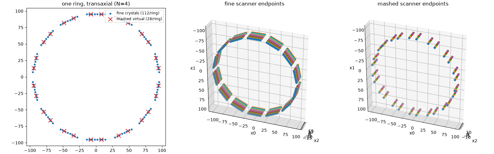
The mashed (virtual) crystals lie at the average position of the within-side blocks they replace. Left: one ring, transaxially – small dots are the fine crystals, large crosses the mashed virtual crystals. Middle / right: all endpoints of the fine and mashed scanners in 3D.
fine_pts = to_numpy_array(scanner.all_lor_endpoints).reshape(
    scanner.num_rings, scanner.num_lor_endpoints_per_ring, 3
)[0]
coarse_pts = to_numpy_array(mash.coarse_scanner.all_lor_endpoints).reshape(
    mash.coarse_scanner.num_rings,
    mash.coarse_scanner.num_lor_endpoints_per_ring,
    3,
)[0]
# transaxial plane = the two axes orthogonal to the symmetry axis
tax = [a for a in range(3) if a != scanner.symmetry_axis]

fig1 = plt.figure(figsize=(16, 5), tight_layout=True)
ax1a = fig1.add_subplot(1, 3, 1)
ax1a.scatter(
    fine_pts[:, tax[0]],
    fine_pts[:, tax[1]],
    s=12,
    color="tab:blue",
    label=f"fine crystals ({fine_pts.shape[0]}/ring)",
)
ax1a.scatter(
    coarse_pts[:, tax[0]],
    coarse_pts[:, tax[1]],
    s=90,
    marker="x",
    color="tab:red",
    label=f"mashed virtual ({coarse_pts.shape[0]}/ring)",
)
ax1a.set_aspect("equal")
ax1a.set_title(f"one ring, transaxial (N={transaxial_factor})")
ax1a.legend(loc="upper right", fontsize="small")

ax1b = fig1.add_subplot(1, 3, 2, projection="3d")
ax1b.view_init(elev=-30, azim=160, roll=180, vertical_axis="y")
scanner.show_lor_endpoints(ax1b, show_linear_index=False)
ax1b.set_title("fine scanner endpoints")

ax1c = fig1.add_subplot(1, 3, 3, projection="3d")
ax1c.view_init(elev=-30, azim=160, roll=180, vertical_axis="y")
mash.coarse_scanner.show_lor_endpoints(ax1c, show_linear_index=False)
ax1c.set_title("mashed scanner endpoints")
fig1.show()
A single view of the central plane, fine vs. mashed
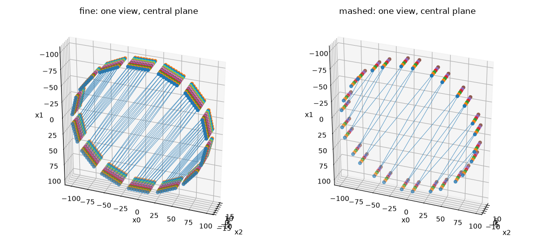
RegularPolygonPETLORDescriptor.show_views() draws the actual LORs for
a set of views and planes. Showing one view of the central plane makes the
LOR thinning explicit: the mashed descriptor has far fewer (and longer,
averaged) LORs for the same projection angle.
central_fine = xp.asarray([num_rings // 2], device=dev)
central_coarse = xp.asarray([num_rings // (2 * axial_factor)], device=dev)
view_fine = xp.asarray([lor_desc.num_views // 4], device=dev)
view_coarse = xp.asarray([coarse_desc.num_views // 4], device=dev)

figv = plt.figure(figsize=(11, 5), tight_layout=True)
axv1 = figv.add_subplot(1, 2, 1, projection="3d")
axv1.view_init(elev=-30, azim=160, roll=180, vertical_axis="y")
scanner.show_lor_endpoints(axv1, show_linear_index=False)
lor_desc.show_views(axv1, views=view_fine, planes=central_fine, lw=0.5)
axv1.set_title("fine: one view, central plane")
axv2 = figv.add_subplot(1, 2, 2, projection="3d")
axv2.view_init(elev=-30, azim=160, roll=180, vertical_axis="y")
mash.coarse_scanner.show_lor_endpoints(axv2, show_linear_index=False)
coarse_desc.show_views(axv2, views=view_coarse, planes=central_coarse, lw=0.5)
axv2.set_title("mashed: one view, central plane")
figv.show()
The two Michelograms (axial plane layout)
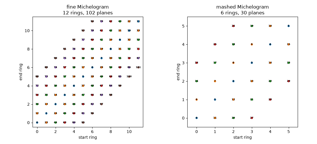
Axial mashing (M) merges neighbouring rings, so the mashed scanner has
fewer rings and therefore a smaller Michelogram – i.e. fewer sinogram planes.
Left: the fine span-1 Michelogram; right: the mashed one.
figmg, axmg = plt.subplots(1, 2, figsize=(11, 5), tight_layout=True)
lor_desc.show_michelogram(axmg[0])
axmg[0].set_title(
    f"fine Michelogram\n{scanner.num_rings} rings, {lor_desc.num_planes} planes"
)
coarse_desc.show_michelogram(axmg[1])
axmg[1].set_title(
    f"mashed Michelogram\n{mash.coarse_scanner.num_rings} rings, "
    f"{coarse_desc.num_planes} planes"
)
figmg.show()
Mash a (simulated) emission sinogram
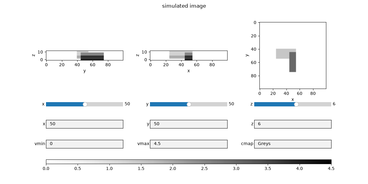
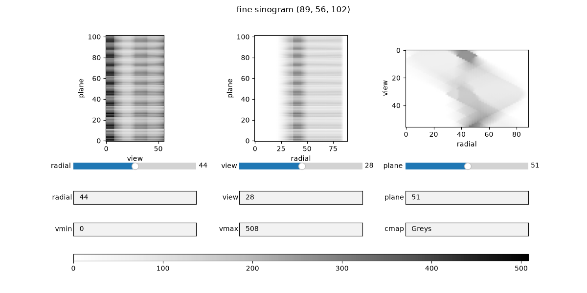
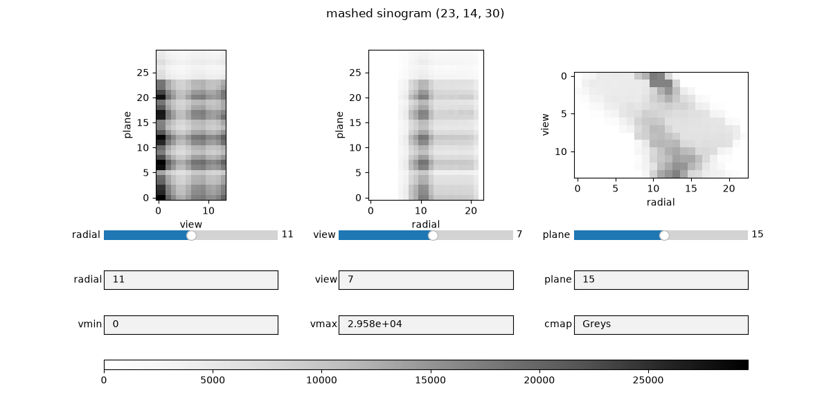
Forward-project a simple phantom through the fine projector to get a fine
emission sinogram, then mash it with mode="sum" (counts add).
(By default coarse_radial_trim is derived as
lor_desc.radial_trim // transaxial_factor so the coarse radial extent
matches the fine data. With coarse_radial_trim=0 the coarse sinogram
would keep extra peripheral radial bins that have no fine contributor – they
would stay empty and the mashed sinogram would appear to lose counts at the
largest radial offsets.)
img_shape = (100, 100, num_rings)
voxel_size = (3.5, 3.5, 3.5)
proj_fine = parallelproj.projectors.RegularPolygonPETProjector(
    lor_desc, img_shape, voxel_size
)

img = xp.zeros(img_shape, dtype=xp.float32, device=dev)
img[25:55, 40:55, 2:] = 1.0
img[45:55, 45:75, :-2] = 2.0
img[:, :, : num_rings // 2] *= 1.5
img[:, :, ::2] *= 1.5

fine_sino = proj_fine(img)
mashed_sino = mash(fine_sino)

# show the image used to simulated the sinograms
_, _, _ = show_vol_cuts(img, fig_title="simulated image")

# The sinograms are 3D arrays.  ``show_vol_cuts`` shows orthogonal cuts with a
# slider per axis, so you can scroll through radial, view and plane.


def _canonical(sino, desc):
    """Return the sinogram as a ``(radial, view, plane)`` numpy array."""
    s = to_numpy_array(sino)
    return np.moveaxis(
        s, (desc.radial_axis_num, desc.view_axis_num, desc.plane_axis_num), (0, 1, 2)
    )


_labels = ("radial", "view", "plane")
_keep = []  # keep references so the interactive slider callbacks are not GC'd

_keep.append(
    show_vol_cuts(
        _canonical(fine_sino, lor_desc),
        axis_labels=_labels,
        fig_title=f"fine sinogram {mash.in_shape}",
        cmap="Greys",
    )
)
_keep.append(
    show_vol_cuts(
        _canonical(mashed_sino, coarse_desc),
        axis_labels=_labels,
        fig_title=f"mashed sinogram {mash.out_shape}",
        cmap="Greys",
    )
)
How many fine LORs does each mashed LOR combine?
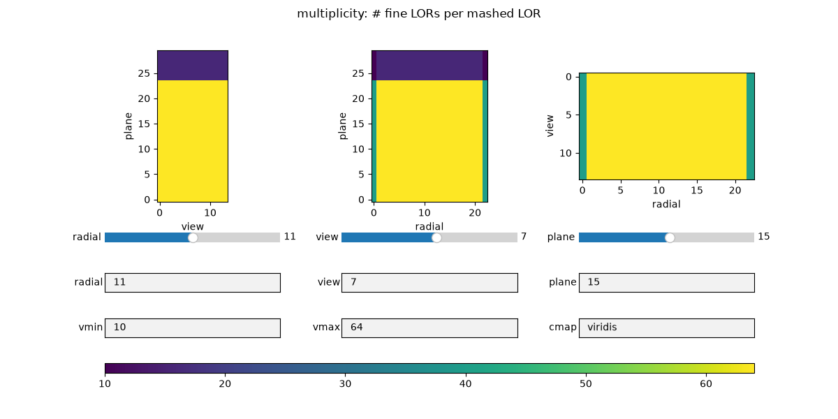
Mashing a sinogram of ones (mode="sum") yields, per mashed bin, the number
of fine LORs that fold into it – its multiplicity. It is largest in the
interior (~ transaxial_factor**2 * axial_factor**2) and smaller toward the
radial / axial edges, where fewer fine LORs contribute.
ones_fine = xp.ones(lor_desc.spatial_sinogram_shape, dtype=xp.float32, device=dev)
multiplicity_sino = mash(ones_fine)  # sum mode -> per-mashed-bin count

_keep.append(
    show_vol_cuts(
        _canonical(multiplicity_sino, coarse_desc),
        axis_labels=_labels,
        fig_title="multiplicity: # fine LORs per mashed LOR",
        cmap="viridis",
    )
)
Fast coarse projector vs. the exact mashed model
A projector built on mash.coarse_lor_descriptor projects directly along
the averaged LORs (cheap). With mode="average" it approximates the
averaged bundle of fine LORs, i.e. mash_avg(P_fine(x)) ~ P_coarse(x). The
two are not identical – a single averaged LOR has a slightly narrower
sensitivity profile than the bundle it replaces – so they agree up to a
resolution-dependent difference (shown below). Use the exact mash(P_fine)
model when that difference matters, and the fast coarse projector otherwise.
mash_avg = parallelproj.pet_lors.SinogramMashingOperator(
    lor_desc,
    transaxial_factor=transaxial_factor,
    axial_factor=axial_factor,
    mode="average",
)
proj_coarse = parallelproj.projectors.RegularPolygonPETProjector(
    mash_avg.coarse_lor_descriptor, img_shape, voxel_size
)

exact = mash_avg(proj_fine(img))  # mash the fine forward projection
fast = proj_coarse(img)  # project directly along the averaged LORs

rel = float(
    np.linalg.norm(to_numpy_array(exact) - to_numpy_array(fast))
    / np.linalg.norm(to_numpy_array(fast))
)
print(
    f"relative difference  ||mash_avg(P_fine x) - P_coarse x|| / ||P_coarse x|| = {rel:.3f}"
)

exact_c = _canonical(exact, mash_avg.coarse_lor_descriptor)
fast_c = _canonical(fast, mash_avg.coarse_lor_descriptor)
_vmax = float(max(exact_c.max(), fast_c.max()))
_keep.append(
    show_vol_cuts(
        exact_c,
        axis_labels=_labels,
        vmin=0,
        vmax=_vmax,
        fig_title="exact:  mash_avg(P_fine x)",
        cmap="Greys",
    )
)
_keep.append(
    show_vol_cuts(
        fast_c,
        axis_labels=_labels,
        vmin=0,
        vmax=_vmax,
        fig_title="fast:   P_coarse x",
        cmap="Greys",
    )
)
_keep.append(
    show_vol_cuts(
        exact_c - fast_c,
        axis_labels=_labels,
        fig_title="difference (exact - fast)",
        cmap="RdBu",
    )
)
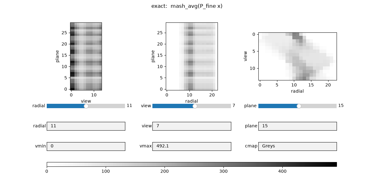
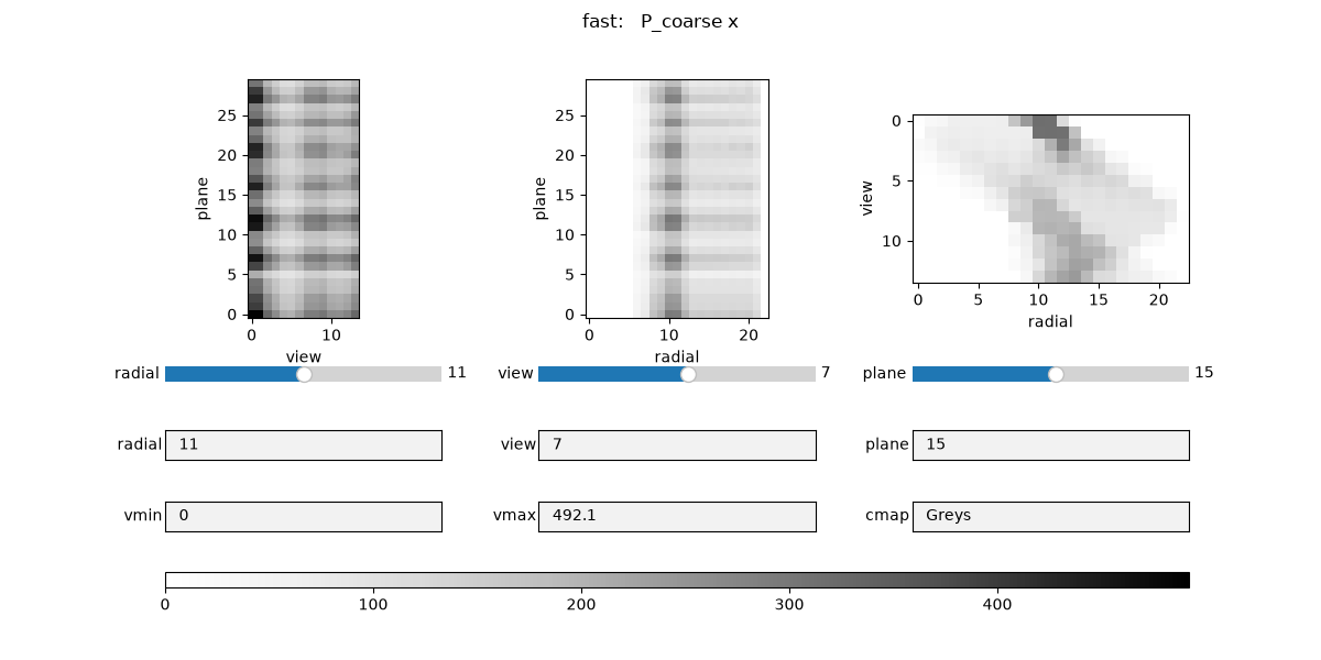
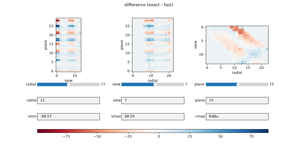
relative difference ||mash_avg(P_fine x) - P_coarse x|| / ||P_coarse x|| = 0.098
Upsampling a coarse sinogram back to the fine grid
Sometimes a quantity is estimated cheaply on the coarse grid (a classic example is the scatter expectation) but the reconstruction runs on the fine grid, so it must be upsampled. The mashing operator’s adjoint does this with no extra dependency – and the mode picks the normalisation:
mash_sum.adjointreplicates: every fine bin gets its coarse bin’s value unchanged. This preserves the per-LOR value/rate (each fine LOR inherits the coarse value) but does not conserve the total – the sum grows by roughly the mashing factor. Use this for rate-like quantities such as a scatter estimate or a forward model.mash_avg.adjointspreads: every fine bin getscoarse / multiplicity. This conserves the total counts (the fine bins of a group sum back to the coarse value) but lowers the per-bin value. Use this for counts you want to redistribute.
Note
To upsample a coarse sinogram back to the fine grid, use the operator’s
adjoint. The adjoint is not the inverse – mashing discards
information, so mash.adjoint(mash(x)) != x. Choose the mode by what you
want to keep: the mode="sum" adjoint replicates the coarse value
into every fine bin (per-bin value/rate preserved, total grows ~ mashing
factor), while the mode="average" adjoint spreads it
(coarse / multiplicity; total counts preserved, per-bin value lowered).
(Interpolation is another option for smooth quantities like scatter, but the array API standard has no interpolation primitive; you would hand-roll linear interpolation or briefly drop to NumPy/SciPy. The two adjoints below are array-API compliant and need nothing extra.)
coarse = mash(fine_sino)  # a coarse (counts) sinogram to upsample
up_replicate = mash.adjoint(coarse)  # sum-mode adjoint: copy (rate-preserving)
up_spread = mash_avg.adjoint(
    coarse
)  # average-mode adjoint: /multiplicity (count-preserving)

print(f"sum(coarse)                  = {float(xp.sum(coarse)):.1f}")
print(
    f"sum(replicate, sum-adjoint)  = {float(xp.sum(up_replicate)):.1f}  (total NOT preserved)"
)
print(
    f"sum(spread, average-adjoint) = {float(xp.sum(up_spread)):.1f}  (total preserved)"
)

_keep.append(
    show_vol_cuts(
        _canonical(up_replicate, lor_desc),
        axis_labels=_labels,
        cmap="Greys",
        fig_title="upsampled: mash.adjoint (replicate, per-bin value preserved)",
    )
)
_keep.append(
    show_vol_cuts(
        _canonical(up_spread, lor_desc),
        axis_labels=_labels,
        cmap="Greys",
        fig_title="upsampled: mash_avg.adjoint (spread, total counts preserved)",
    )
)
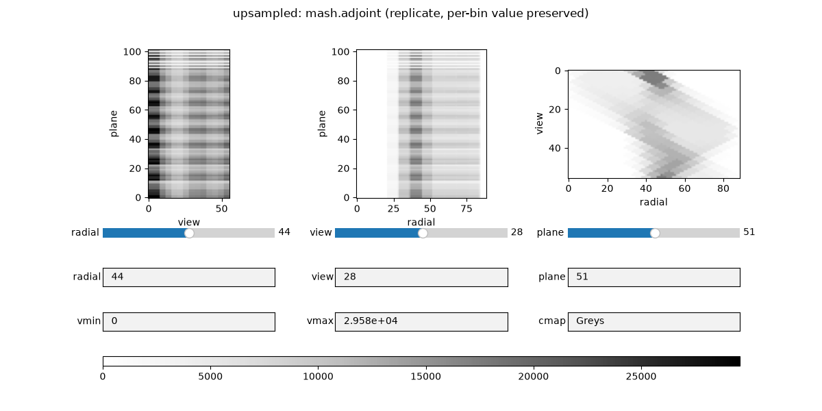
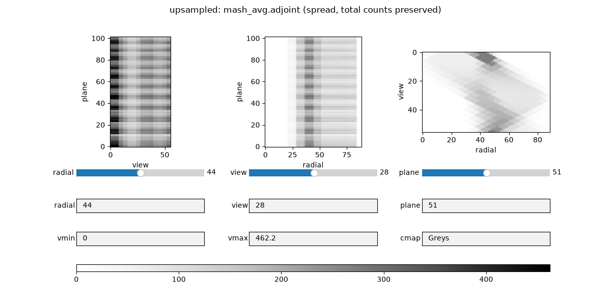
sum(coarse)                  = 42456424.0
sum(replicate, sum-adjoint)  = 2594081280.0  (total NOT preserved)
sum(spread, average-adjoint) = 42456428.0  (total preserved)
Mashing GE-layout sinograms (by composition)
GE sinograms use the “span-3 in the centre” staircase segmentation (segment 0
pools ring differences {-1, 0, +1} into direct/cross planes, oblique
segments pool {+/-2k, +/-(2k+1)}). SinogramMashingOperator itself is
span-1 only, but GE mashing follows cleanly by composition, and the result
is a plain span-1 coarse sinogram (no GE cross planes to carry around):
a span-1 <-> GE
SinogramAxialCompressionOperator; itsmode="average"adjoint distributes a GE sinogram back onto the span-1 grid while preserving counts (each cross-plane count is split evenly between its two ring differences);the span-1
SinogramMashingOperatorthen mashes that span-1 sinogram to a coarse span-1 sinogram.
ge_span1 = parallelproj.pet_lors.RegularPolygonPETLORDescriptor(
    scanner,
    parallelproj.pet_lors.Michelogram(scanner.num_rings, max_ring_difference=3, span=1),
    radial_trim=11,
)

# span-1 <-> GE (average mode; its adjoint distributes GE -> span-1)
ge_to_span1 = parallelproj.pet_lors.SinogramAxialCompressionOperator(
    ge_span1, target_layout=parallelproj.pet_lors.MichelogramLayout.GE, mode="average"
)
ge_desc = ge_to_span1.out_lor_descriptor  # the GE data layout

# span-1 detector mashing (same factors as above)
mash_span1 = parallelproj.pet_lors.SinogramMashingOperator(
    ge_span1, transaxial_factor=transaxial_factor, axial_factor=axial_factor, mode="sum"
)
span1_coarse_desc = mash_span1.coarse_lor_descriptor

# GE data --(distribute)--> fine span-1 --(mash)--> coarse span-1
ge_mash = CompositeLinearOperator([mash_span1, ge_to_span1.H])

print(
    f"fine   GE sinogram   : {ge_mash.in_shape}  (layout={ge_desc.michelogram.layout.name})"
)
print(
    f"mashed span-1 sinogram : {ge_mash.out_shape}  "
    f"(coarse rings={mash_span1.coarse_scanner.num_rings}, "
    f"layout={span1_coarse_desc.michelogram.layout.name}, span={span1_coarse_desc.span})"
)
fine   GE sinogram   : (89, 56, 61)  (layout=GE)
mashed span-1 sinogram : (23, 14, 24)  (coarse rings=6, layout=STANDARD, span=1)
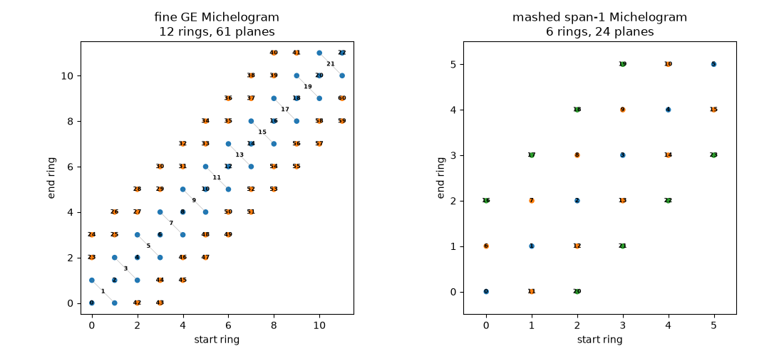
The GE input Michelogram vs the coarse span-1 output Michelogram.
figge, axge = plt.subplots(1, 2, figsize=(11, 5), tight_layout=True)
ge_desc.show_michelogram(axge[0])
axge[0].set_title(
    f"fine GE Michelogram\n{scanner.num_rings} rings, {ge_desc.num_planes} planes"
)
span1_coarse_desc.show_michelogram(axge[1])
axge[1].set_title(
    f"mashed span-1 Michelogram\n{mash_span1.coarse_scanner.num_rings} rings, "
    f"{span1_coarse_desc.num_planes} planes"
)
figge.show()
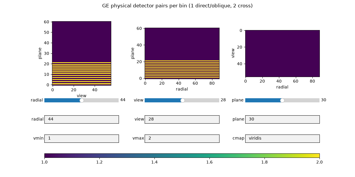
GE detector sensitivity
The projector traces a single representative LOR per plane, so the
segment-0 cross planes (which physically collect two ring differences) are
under-weighted. We multiply the projection by the plane multiplicity
(2 on cross planes, 1 elsewhere) to give the cross planes their true
double sensitivity before mashing.
_plane_mult = to_numpy_array(ge_desc.michelogram.plane_multiplicity).astype("float64")
_bshape = [1, 1, 1]
_bshape[ge_desc.plane_axis_num] = ge_desc.spatial_sinogram_shape[ge_desc.plane_axis_num]
fine_phys_mult = xp.asarray(
    np.broadcast_to(
        _plane_mult.reshape(_bshape), ge_desc.spatial_sinogram_shape
    ).copy(),
    dtype=xp.float64,
    device=dev,
)

_keep.append(
    show_vol_cuts(
        _canonical(fine_phys_mult, ge_desc),
        axis_labels=_labels,
        fig_title="GE physical detector pairs per bin (1 direct/oblique, 2 cross)",
        cmap="viridis",
    )
)
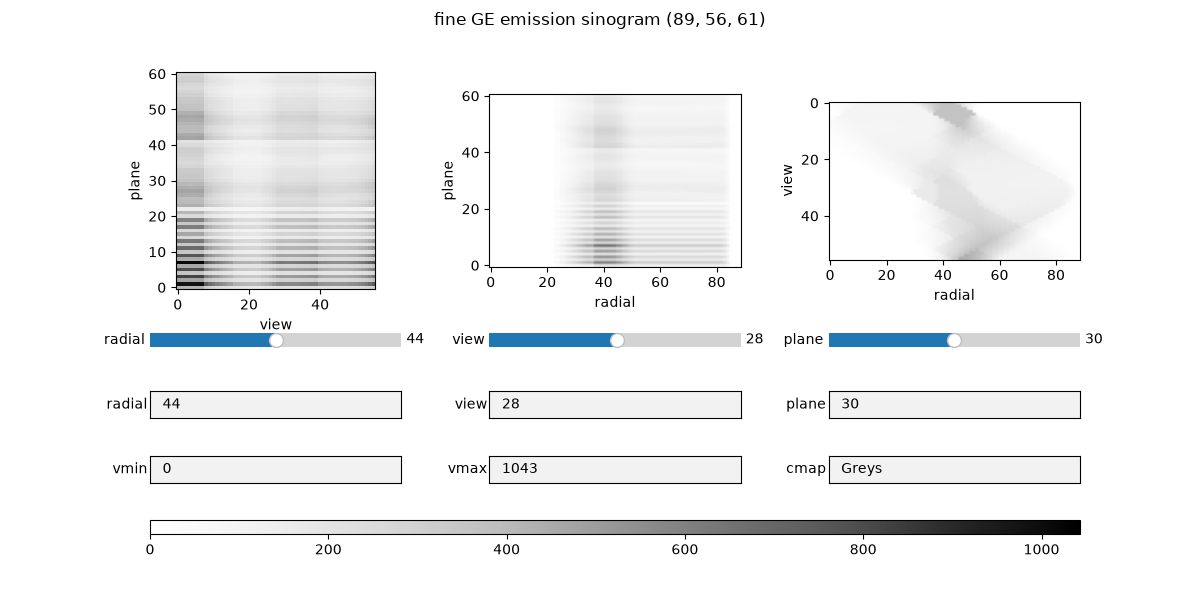
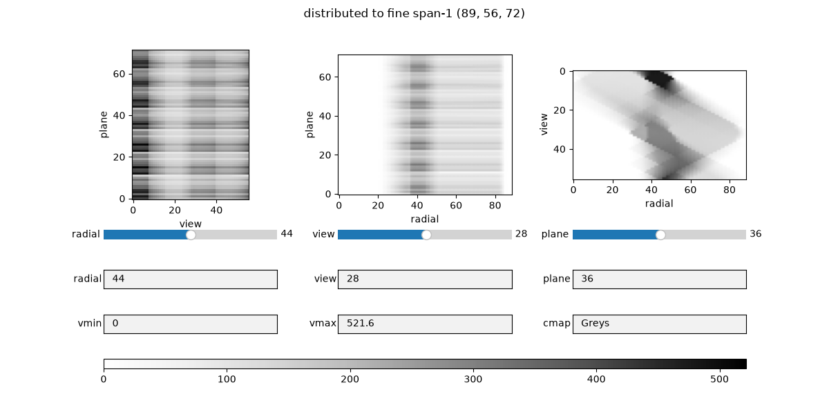
Mash a (simulated) GE emission sinogram
Forward-project the same phantom through the projector (weighted for the cross-plane sensitivity), then apply the composite operator. The pipeline first distributes the GE-style sinogram data onto the fine span-1 grid (the “un-GE” step), then mashes to a coarse span-1 sinogram. Scroll through radial / view / plane.
proj_ge = parallelproj.projectors.RegularPolygonPETProjector(
    ge_desc, img_shape, voxel_size
)
ge_fine_sino = proj_ge(img) * fine_phys_mult  # GE data with cross planes at 2x
span1_fine_sino = ge_to_span1.H(ge_fine_sino)  # distribute GE -> fine span-1
span1_coarse_sino = ge_mash(ge_fine_sino)  # = mash_span1(span1_fine_sino)

_keep.append(
    show_vol_cuts(
        _canonical(ge_fine_sino, ge_desc),
        axis_labels=_labels,
        fig_title=f"fine GE emission sinogram {tuple(ge_mash.in_shape)}",
    )
)
_keep.append(
    show_vol_cuts(
        _canonical(span1_fine_sino, ge_span1),
        axis_labels=_labels,
        fig_title=f"distributed to fine span-1 {tuple(ge_span1.spatial_sinogram_shape)}",
    )
)
_keep.append(
    show_vol_cuts(
        _canonical(span1_coarse_sino, span1_coarse_desc),
        axis_labels=_labels,
        fig_title=f"mashed coarse span-1 sinogram {tuple(ge_mash.out_shape)}",
    )
)

# counts are preserved end to end (distribute preserves, sum-mash preserves)
print(
    f"sum(fine GE)          = {float(xp.sum(ge_fine_sino)):.1f}\n"
    f"sum(mashed span-1)    = {float(xp.sum(span1_coarse_sino)):.1f}  (counts preserved)"
)
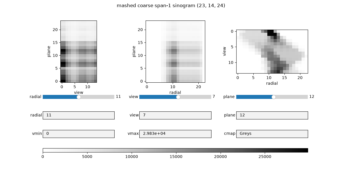
sum(fine GE)          = 29917315.4
sum(mashed span-1)    = 29917315.4  (counts preserved)
Upsample the coarse span-1 sinogram back to the fine span-1 grid
As before, the span-1 mashing operator’s adjoint upsamples the coarse
sinogram. Since it was pooled by sum, the count-preserving upsampling is
the average-mode adjoint, which spreads each coarse bin over its fine bins.
mash_span1_avg = parallelproj.pet_lors.SinogramMashingOperator(
    ge_span1,
    transaxial_factor=transaxial_factor,
    axial_factor=axial_factor,
    mode="average",
)
span1_upsampled = mash_span1_avg.adjoint(
    span1_coarse_sino
)  # fine span-1, counts preserved

print(
    f"sum(upsampled span-1) = {float(xp.sum(span1_upsampled)):.1f}  "
    f"(matches sum(mashed span-1) = {float(xp.sum(span1_coarse_sino)):.1f})"
)

_keep.append(
    show_vol_cuts(
        _canonical(span1_upsampled, ge_span1),
        axis_labels=_labels,
        fig_title=f"upsampled span-1 sinogram (avg-adjoint, {tuple(ge_span1.spatial_sinogram_shape)})",
    )
)
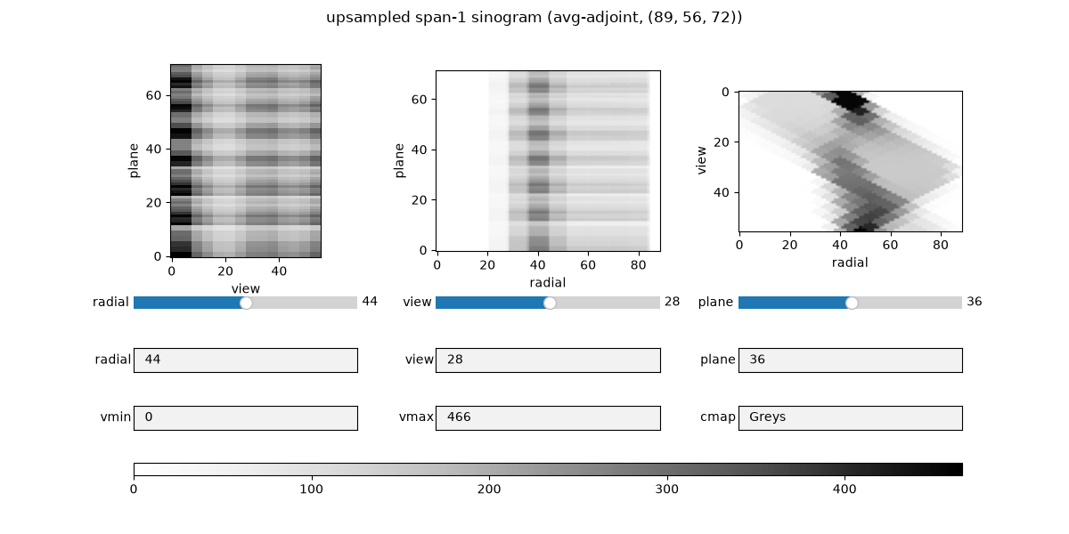
sum(upsampled span-1) = 29917315.4 (matches sum(mashed span-1) = 29917315.4)
Round trip: back to the original fine GE sinogram
Finally, return to the original GE layout. Re-combining span-1 -> GE is the
sum-mode span-1 <-> GE operator’s forward (each GE cross plane sums its two
span-1 planes, exactly undoing the earlier mode="average" distribution).
We fold the upsampling and re-combination into a single operator that maps the
coarse span-1 sinogram straight back to fine GE:
coarse span-1 –(avg-adjoint of the mash)–> fine span-1 –(sum span-1 -> GE)–> fine GE
Counts are preserved; the result approximates the original fine GE sinogram up to the axial/transaxial resolution lost in mashing.
ge_recombine = parallelproj.pet_lors.SinogramAxialCompressionOperator(
    ge_span1, target_layout=parallelproj.pet_lors.MichelogramLayout.GE, mode="sum"
)
coarse_span1_to_ge = CompositeLinearOperator([ge_recombine, mash_span1_avg.H])

ge_reconstructed = coarse_span1_to_ge(span1_coarse_sino)  # fine GE (approx)

rel_ge = float(
    np.linalg.norm(to_numpy_array(ge_reconstructed) - to_numpy_array(ge_fine_sino))
    / np.linalg.norm(to_numpy_array(ge_fine_sino))
)
print(
    f"sum(upsampled sino) = {float(xp.sum(ge_reconstructed)):.1f}  (counts preserved)\n"
    f"rel. difference to original fine GE = {rel_ge:.2f}  (resolution lost in mashing)"
)

_keep.append(
    show_vol_cuts(
        _canonical(ge_reconstructed, ge_desc),
        axis_labels=_labels,
        fig_title=f"upsampled sinogram (GE plane layout ) {tuple(ge_desc.spatial_sinogram_shape)}",
    )
)

plt.show()
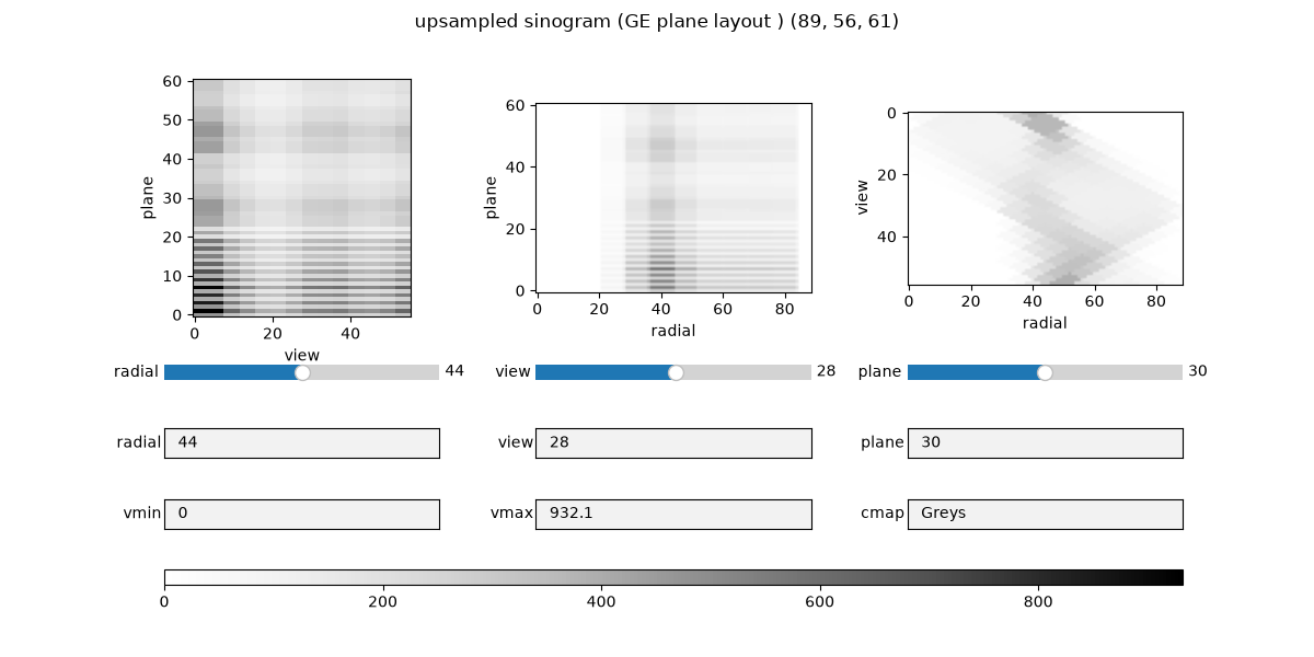
sum(upsampled sino) = 29917315.4  (counts preserved)
rel. difference to original fine GE = 0.13  (resolution lost in mashing)
Total running time of the script: (0 minutes 15.306 seconds)