PET LOR / sinogram descriptors `parallelproj.pet_lors`¶

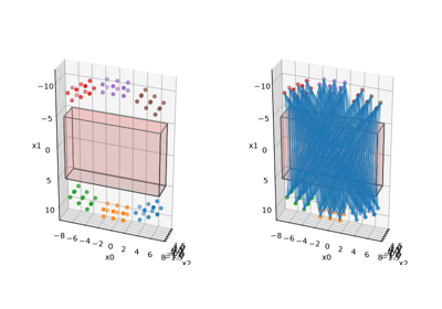
Non-TOF and TOF projections using a modularized (block) PET scanner geometry

Parameters:

scanner (ModularizedPETScannerGeometry) – A modularized PET scanner consisting of block modules with the same number of LOR endpoints.
all_block_pairs (Array) – An array containing pairs of integer numbers encoding which block pairs are in coincidence and form valid LORs.

Examples

Non-TOF and TOF projections using a modularized (block) PET scanner geometry

property all_block_pairs: Array¶: all block pairs in coincidence

property dev: str¶: device to use for storing the LOR endpoints

get_lor_coordinates(block_pair_nums: None | Array = None) → tuple[Array, Array][source]¶

Get the coordinates of LORs for the given block pair numbers.

Parameters:

block_pair_nums (None or Array, optional) – The block pair numbers for which to retrieve the LOR coordinates. If None, all block pair numbers will be used.

Returns:

tuple[Array, Array]
A tuple containing two arrays –
- the start coordinates of the LORs, with shape (N, 3), where N is the total number of LORs.
- the end coordinates of the LORs, with shape (N, 3)

Return type:

tuple[Array, Array]

Examples

property num_block_pairs: int¶: number of block pairs in coincidence

property num_lorendpoints_per_block: int¶: number of LOR endpoints per block

property num_lors_per_block_pair: int¶: number of LORs per block pair

property scanner: ModularizedPETScannerGeometry¶: the scanner for which coincidences are described

show_block_pair_lors(ax: Axes, block_pair_nums: Array, lw: float = 0.2, **kwargs) → None[source]¶

show all LORs connecting all endpoints between blocks forming a block pairs

Parameters:

ax (plt.Axes) – a 3D matplotlib axes
block_pair_nums (Array) – Integer array of block pair indices to show.
lw (float, optional) – the line width, by default 0.2

Return type:

None

Examples

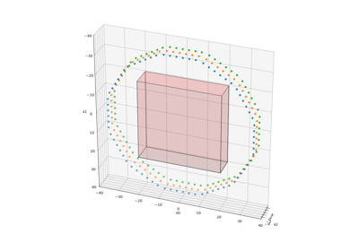
Non-TOF and TOF projections using a modularized (block) PET scanner geometry

property xp: ModuleType¶: array module to use for storing the LOR endpoints

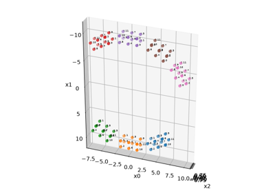
class parallelproj.pet_lors.LOREndpointOrder(*values)[source]¶

Bases: Enum

Which physical endpoint of each LOR is the start (xstart) vs the end (xend).

Non-TOF projections are unaffected (an LOR is geometrically symmetric). For TOF, the TOF-bin axis is defined along xstart -> xend, so swapping the endpoints reverses the TOF bins (bin k <-> bin num_tofbins - 1 - k). Use this to match a given vendor’s start/end – and hence TOF-bin – convention.

Note

TOFParameters.tofcenter_offset is measured along xstart -> xend and is not adjusted automatically. If you combine a non-zero tofcenter_offset with END_START, negate the offset yourself.

Examples

END_START = 2¶

xstart and xend are exchanged for every LOR.

Examples

START_END = 1¶

xstart is the descriptor’s start endpoint (default; original behaviour).

Examples

classmethod __getitem__(name)¶

Return the member matching name.

Examples

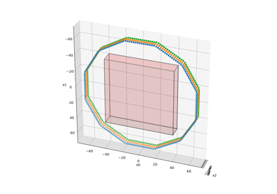
class parallelproj.pet_lors.Michelogram(num_rings: int, max_ring_difference: int, span: int = 1, layout: MichelogramLayout = MichelogramLayout.STANDARD, segment_order: SegmentOrder = SegmentOrder.POSITIVE_FIRST)[source]¶

Bases: object

Axial plane layout for a cylindrical PET scanner under odd span.

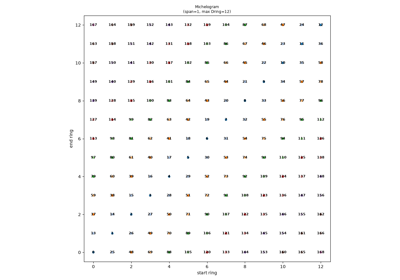
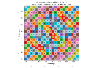
Encapsulates the segment / axial-position combinatorics that map every valid ring pair \((s, e)\) onto a sinogram plane index under span conventions.

For span \(S\) (odd) and a maximum ring difference \(D\), each ring pair with \(|e - s| \le D\) is assigned a segment via ring_diff_to_segment(). Ring pairs sharing the same \((\text{segment},\; s + e)\) collapse into a single plane. Planes are ordered by \((|\text{seg}|,\; -\text{seg},\; s + e)\) \([0, +1, -1, +2, -2, \ldots]\) with axial bins increasing in \(s + e\) (equivalently in z for equispaced rings).

The class knows nothing about ring z-positions, scanner radius, or sinogram axis ordering – it operates on pure integer indices. Consumers (e.g. RegularPolygonPETLORDescriptor, SinogramAxialCompressionOperator) combine it with the geometry- and array-API-specific information they need.

For span = 1 the layout reduces to the unspanned Michelogram (each ring pair is its own plane with max_multiplicity == 1); the ordering rd = 0, +1, -1, +2, -2, ... with each ring difference sorted by ring sum.

Parameters:

num_rings (int) – Number of detector rings (\(R \ge 1\)).
max_ring_difference (int) – Maximum ring difference \(|e - s|\) considered (\(\ge 0\)). Values larger than num_rings - 1 have no extra effect.
span (int, optional) – Axial compression factor – must be odd and \(\ge 1\). Default 1 (no compression). Ignored (and reported as None) for layout=MichelogramLayout.GE.
layout (MichelogramLayout, optional) – Axial plane layout / segmentation convention, by default MichelogramLayout.STANDARD. See MichelogramLayout.
segment_order (SegmentOrder, optional) – Order of the signed oblique segments, by default SegmentOrder.POSITIVE_FIRST (0, +1, -1, +2, -2, ...). Use SegmentOrder.NEGATIVE_FIRST for 0, -1, +1, -2, +2, .... This only permutes the sinogram planes; segment numbering and plane counts are unchanged. See SegmentOrder.

Examples

>>> m = Michelogram(num_rings=3, max_ring_difference=2, span=3)
>>> int(m.num_planes)
7
>>> int(m.max_multiplicity)
2
>>> int(m.ring_diff_to_segment(0)), int(m.ring_diff_to_segment(2)),         int(m.ring_diff_to_segment(-2))
(0, 1, -1)
>>> m.plane_segment.tolist()  # POSITIVE_FIRST (default): +1 before -1
[0, 0, 0, 0, 0, 1, -1]
>>> m2 = Michelogram(3, 2, span=3, segment_order=SegmentOrder.NEGATIVE_FIRST)
>>> m2.plane_segment.tolist()  # NEGATIVE_FIRST: -1 before +1
[0, 0, 0, 0, 0, -1, 1]

Examples

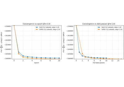
Convergence comparison: SGD vs SVRG with logcosh regularization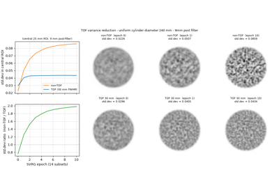

TOF vs non-TOF: variance reduction in a uniform cylinder

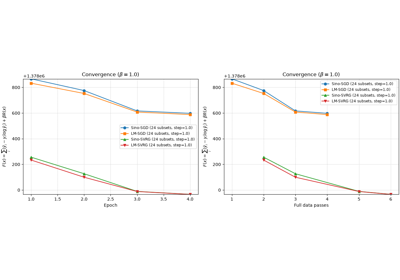
Convergence comparison: SGD vs SVRG with regularization (sinogram and listmode)

PDHG and LM-SPDHG to optimize the Poisson logL and total variation

Transmission reconstruction: MLTR, SPS and L-BFGS-B

Accelerating MLTR with ordered subsets (OS-MLTR) and SVRG

Penalised transmission reconstruction (MAPTR) with an edge-preserving prior

Joint activity and attenuation reconstruction (MLAA) for TOF PET

average_z_per_plane(ring_positions) → tuple[ndarray, ndarray][source]¶

Mean ring z-coordinate per plane, separately for start and end rings.

Equivalent to averaging ring_positions over the contributing ring pairs of each plane. For span =1 planes this is trivially the single contributing ring’s z; for span > 1 planes it produces the averaged-LOR z-position used by the spanned setup of RegularPolygonPETLORDescriptor and by show_segment_lors().

Parameters:

ring_positions (array-like, shape (num_rings,)) – z-coordinate of each ring (any backend; converted via np.asarray).

Returns:

start_z (np.ndarray, shape (num_planes,), dtype float32)
end_z (np.ndarray, shape (num_planes,), dtype float32)

Return type:

tuple[ndarray, ndarray]

Examples

compression_index_maps(target_span: int) → tuple[ndarray, ndarray, ndarray, ndarray][source]¶

Build gather/scatter index maps to a higher-span Michelogram.

Convenience wrapper around compression_index_maps_to() that builds the target Michelogram internally as Michelogram(self.num_rings, self.max_ring_difference, span=target_span, segment_order=self.segment_order) (the segment ordering is inherited from self).

Parameters:: target_span (int) – Odd integer >= self.span; additionally (target_span // self.span) must be odd.
Return type:: See compression_index_maps_to().
Raises:: ValueError – If target_span is not a positive odd integer. Further validation errors are raised by compression_index_maps_to().

Examples

compression_index_maps_to(target: Michelogram) → tuple[ndarray, ndarray, ndarray, ndarray][source]¶

Build gather/scatter index maps to a pre-built target Michelogram.

Returns the integer index structures needed to map planes of this Michelogram onto planes of target.

Both Michelograms must describe the same scanner geometry (target.num_rings == self.num_rings), and target.span must be an integer multiple of self.span. Because both spans are odd by construction, the ratio target.span / self.span is then automatically odd, which guarantees that every ring pair of any input plane shares the same target plane – so the operation is a single-valued gather.

The target’s max_ring_difference must be at least self.max_ring_difference so every input ring pair has a target plane. If it is strictly greater, the resulting maps still work but some output planes will have zero multiplicity (output bins that no input ring pair contributes to).

Parameters:

target (Michelogram) – Pre-built target Michelogram. Validation rules above.

Returns:

target_for_p1 (np.ndarray, shape (self.num_planes,), dtype int64) – For each plane of this Michelogram, the corresponding plane index in target.
idx2d (np.ndarray, shape (target.num_planes, target_max_mult), int64) – For each target plane, the indices in this Michelogram that contribute, right-padded with 0. Use mask to filter.
mask (np.ndarray, same shape as idx2d, dtype float32) – 1.0 for valid entries, 0.0 for right-padding.
target_multiplicity (np.ndarray, shape (target.num_planes,), int32) – Number of self-planes folded into each target plane.

Raises:

TypeError – If target is not a Michelogram instance.
ValueError – If target.num_rings differs from self.num_rings; if target.span < self.span; if self.span does not divide target.span; or if target.max_ring_difference < self.max_ring_difference.

Return type:

tuple[ndarray, ndarray, ndarray, ndarray]

Examples

classmethod ge(num_rings: int, max_ring_difference: int, segment_order: SegmentOrder = SegmentOrder.POSITIVE_FIRST) → Michelogram[source]¶

Convenience constructor for the GE-style layout.

Equivalent to Michelogram(num_rings, max_ring_difference, layout=MichelogramLayout.GE, segment_order=segment_order). See MichelogramLayout for the segmentation definition and SegmentOrder for the segment ordering.

Examples

Parameters:

num_rings (int)
max_ring_difference (int)
segment_order (SegmentOrder)

Return type:

Michelogram

property layout: MichelogramLayout¶: Axial plane layout convention (STANDARD or GE).

property max_multiplicity: int¶: Largest plane multiplicity (most ring pairs in any one plane).

property max_ring_difference: int¶: Maximum ring difference \(|e - s|\).

property num_planes: int¶: Total number of sinogram planes.

property num_rings: int¶: Number of rings.

property parent_plane_indices: ndarray | None¶

Plane indices of this michelogram’s planes in the parent it was derived from, shape (num_planes,), dtype int64 – or None for a normally-constructed Michelogram.

Set only by select_segments(): entry k is the plane index that restricted plane k had in the full michelogram, so a full sinogram can be reduced to the restricted one with full_sino[..., parent_plane_indices, ...] along the plane axis.

property plane_axial_midpoint_int: ndarray¶: Integer axial midpoint \(s + e\) (= twice the actual midpoint) for each plane, shape (num_planes,), dtype int32.

property plane_end_rings: ndarray¶

Contributing end ring indices per plane, right-padded with 0.

Shape (num_planes, max_multiplicity), dtype int32. Use plane_mask to identify the valid entries.

plane_for_ring_pair(s: int, e: int) → int[source]¶

Plane index for the ring pair (s, e).

Raises:

IndexError – If either s or e is outside [0, num_rings).
ValueError – If \(|e - s| > \text{max\_ring\_difference}\).

Parameters:

s (int)
e (int)

Return type:

int

Examples

property plane_for_ring_pair_table: ndarray¶: (num_rings, num_rings) lookup table whose entry [s, e] is the plane index for ring pair (s, e), or -1 if \(|e - s| > \text{max\_ring\_difference}\).

property plane_mask: ndarray¶

Validity mask for plane_start_rings / plane_end_rings.

Shape (num_planes, max_multiplicity), dtype float32. Entries are 1.0 for valid contributing ring pairs and 0.0 for right-padding.

property plane_multiplicity: ndarray¶: Number of ring pairs contributing to each plane, shape (num_planes,), dtype int32.

property plane_segment: ndarray¶: Signed segment number for each plane, shape (num_planes,), dtype int32.

property plane_start_rings: ndarray¶

Contributing start ring indices per plane, right-padded with 0.

Shape (num_planes, max_multiplicity), dtype int32. Use plane_mask to identify the valid entries.

ring_diff_to_segment(rd: int) → int[source]¶

Signed segment number for a given ring difference \(e - s\).

For the STANDARD layout: 0 if \(|rd| \le \text{half\_span}\), otherwise \(\pm k\) with \(k = \lceil (|rd| - \text{half\_span}) / S \rceil\) and the sign of \(rd\).

For the GE layout: 0 if \(|rd| \le 1\), otherwise \(\pm k\) with \(k = \lfloor |rd| / 2 \rfloor\) (so each oblique segment holds the ring-difference pair \(\{2k, 2k+1\}\)) and the sign of \(rd\).

Examples

Parameters:: rd (int)
Return type:: int

property segment_order: SegmentOrder¶: Order of the signed oblique segments (POSITIVE_FIRST or NEGATIVE_FIRST).

select_segments(segments: Sequence[int]) → Michelogram[source]¶

Return a new Michelogram keeping only the given segments.

max_ring_difference / span / layout still define the segmentation; segments selects which of the resulting signed segments to keep. The selection is treated as a set – plane ordering remains governed by segment_order, so the restricted michelogram is the order-preserving subsequence of this one, with plane indices renumbered 0 .. K-1. Segment labels are unchanged (e.g. select_segments([1]) yields planes whose plane_segment is still 1, not 0).

The result exposes parent_plane_indices (the plane index each kept plane had here), enabling gather/scatter between the full and restricted sinograms (see SinogramSegmentSelectionOperator).

Parameters:

segments (Sequence[int]) – Signed segment numbers to keep. Order and duplicates are ignored.

Raises:

TypeError – If segments is not a sequence of ints (e.g. a bare int).
ValueError – If segments is empty or contains a segment that does not exist for this michelogram.

Return type:

Michelogram

Examples

show(ax: Axes, show_merge_lines: bool = True, plane_index_fontsize: float = 6, **kwargs) → None[source]¶

Draw the Michelogram scatter plot onto ax.

Each point represents a valid ring pair (s, e), colored by abs(segment). For span > 1, ring pairs that share the same (segment, s + e) and therefore collapse into the same sinogram plane are connected by a thin grey line when show_merge_lines is True.

Parameters:

ax (plt.Axes) – 2-D matplotlib axes (not 3-D).
show_merge_lines (bool, optional) – Draw lines connecting ring pairs that merge into the same plane. Defaults to True. Only has a visible effect for span > 1.
plane_index_fontsize (float, optional) – Font size of the per-plane index annotations placed at each ring-pair (or merged-group) centroid. Defaults to 6. Useful knob when the Michelogram is large (lower to avoid overlap) or small (raise for readability).
**kwargs – Forwarded to ax.scatter (e.g. s=4, cmap="RdBu_r").

Return type:

None

Examples

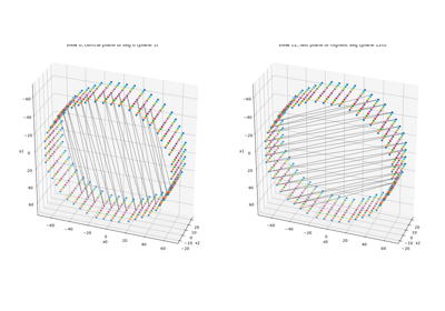
show_segment_lors(ring_positions, axs=None, uncompressed_lor_kwargs: dict | None = None, compressed_lor_kwargs: dict | None = None, inset_plane_index_fontsize: float = 4)[source]¶

Side-view LOR diagram per segment with a Michelogram inset.

Mirrors the descriptor’s RegularPolygonPETLORDescriptor.show_segment_lors(), but takes ring_positions explicitly so the Michelogram can be visualised standalone (e.g. with np.arange(num_rings) for a purely schematic plot, or with the user’s actual ring z-positions).

Subplots are arranged in a 2-row grid (when negative segments exist):

columns indexed by abs(segment): 0, 1, 2, …
row 0 non-negative segments (0, +1, +2, …)
row 1, col 0 Michelogram inset
row 1, col >= 1 negative segments (-1, -2, …)

Each LOR subplot shows the uncompressed (per-ring-pair) LORs as solid black lines and the compressed (axially-averaged) LORs as dashed coloured lines.

Parameters:

ring_positions (array-like, shape (num_rings,)) – z-coordinate of each ring.
axs (2-D array-like of Axes, optional) – Pre-existing axes of shape (n_rows, n_cols). If None, a new figure is created.
uncompressed_lor_kwargs (dict, optional) – Style overrides for the uncompressed LOR lines.
compressed_lor_kwargs (dict, optional) – Style overrides for the compressed LOR lines.
inset_plane_index_fontsize (float)

Return type:

matplotlib.figure.Figure

Examples

property span: int | None¶: Axial compression factor (odd), or None for the GE layout.

class parallelproj.pet_lors.MichelogramLayout(*values)[source]¶

Bases: Enum

Axial plane layout / segmentation convention for a Michelogram.

Examples

GE = 2¶

GE-style mixed axial layout.

Segment 0 collects ring differences \(\{-1, 0, +1\}\) (the \(\pm 1\) cross planes are summed into virtual direct planes at the intermediate axial positions, exactly as in a Siemens span-3 segment 0), while every oblique segment \(\pm k\) collects the ring-difference pair \(\{\pm 2k, \pm(2k+1)\}\) without combination. Segments are ordered 0, +1, -1, +2, -2, ... with axial positions increasing within each segment. span is ignored for this layout (see Michelogram.span, which returns None). This is the segment (theta) / ring-difference (dZ) plane ordering used by GE-style sinograms (also known as “span 2” in STIR). Combine it with a matching RegularPolygonPETLORDescriptor for the GE scanner of interest.

Examples

STANDARD = 1¶

Siemens/CTI-style layout parameterised by an odd span (default).

Examples

classmethod __getitem__(name)¶

Return the member matching name.

Examples

class parallelproj.pet_lors.PETLORDescriptor(scanner: ModularizedPETScannerGeometry)[source]¶

Bases: ABC

abstract base class to describe which modules / indices in modules of a modularized PET scanner are in coincidence; defining geometrical LORs

Examples

Non-TOF and TOF projections using a modularized (block) PET scanner geometry

Convergence comparison: SGD vs SVRG with logcosh regularization

PDHG and SPDHG for PET reconstruction with a directional TV prior

TOF vs non-TOF: variance reduction in a uniform cylinder

Convergence comparison: SGD vs SVRG with regularization (sinogram and listmode)

Penalised transmission reconstruction (MAPTR) with an edge-preserving prior

Parameters:: scanner (ModularizedPETScannerGeometry) – a modularized PET scanner

Examples

Non-TOF and TOF projections using a modularized (block) PET scanner geometry

Convergence comparison: SGD vs SVRG with logcosh regularization

PDHG and SPDHG for PET reconstruction with a directional TV prior

TOF vs non-TOF: variance reduction in a uniform cylinder

Convergence comparison: SGD vs SVRG with regularization (sinogram and listmode)

Penalised transmission reconstruction (MAPTR) with an edge-preserving prior

property dev: str¶: device to use for storing the LOR endpoints

abstractmethod get_lor_coordinates() → tuple[Array, Array][source]¶

Return the start and end world coordinates of all (or a subset of) LORs.

Subclasses may accept optional keyword arguments to restrict which LORs are returned (e.g. views= for sinogram descriptors, block_pair_nums= for block descriptors). Calling with no arguments always returns all LORs.

Returns:

xstart (Array) – Float array of shape (..., 3) with the world coordinates of the LOR start points. The leading dimensions depend on the concrete subclass: (N, 3) for block-based descriptors, (*spatial_sinogram_shape, 3) for sinogram-based descriptors.
xend (Array) – Float array with the same shape as xstart containing the LOR end points.

Return type:

tuple[Array, Array]

Examples

property scanner: ModularizedPETScannerGeometry¶: the scanner for which coincidences are described

property xp: ModuleType¶: array module to use for storing the LOR endpoints

class parallelproj.pet_lors.RadialDirection(*values)[source]¶

Bases: Enum

Direction in which the sinogram radial (tangential) index increases.

The central radial bin always connects detectors (0, N/2); this enum controls which side of the centre positive radial offsets fall on.

Examples

MINUS = 2¶

Radial index increases with decreasing detector-index difference.

Examples

PLUS = 1¶

Radial index increases with increasing detector-index difference (default).

Examples

classmethod __getitem__(name)¶

Return the member matching name.

Examples

class parallelproj.pet_lors.RegularPolygonPETLORDescriptor(scanner: RegularPolygonPETScannerGeometry, michelogram: Michelogram | None = None, radial_trim: int = 3, sinogram_order: SinogramSpatialAxisOrder = SinogramSpatialAxisOrder.RVP, zig_zag_order: SinogramZigZagOrder = SinogramZigZagOrder.END_FIRST, view_direction: ViewDirection = ViewDirection.PLUS, radial_direction: RadialDirection = RadialDirection.PLUS, lor_endpoint_order: LOREndpointOrder = LOREndpointOrder.START_END, view0_shift: int = 0)[source]¶

Bases: PETLORDescriptor

LOR descriptor for a regular polygon PET scanner where we have coincidences within and between “rings (polygons of modules)” The geometrical LORs can be sorted into a sinogram having a “plane”, “view” and “radial” axis.

Examples

Convergence comparison: SGD vs SVRG with logcosh regularization

PDHG and SPDHG for PET reconstruction with a directional TV prior

TOF vs non-TOF: variance reduction in a uniform cylinder

Convergence comparison: SGD vs SVRG with regularization (sinogram and listmode)

PDHG and LM-SPDHG to optimize the Poisson logL and total variation

Transmission reconstruction: MLTR, SPS and L-BFGS-B

Accelerating MLTR with ordered subsets (OS-MLTR) and SVRG

Penalised transmission reconstruction (MAPTR) with an edge-preserving prior

Joint activity and attenuation reconstruction (MLAA) for TOF PET

Parameters:

scanner (RegularPolygonPETScannerGeometry) – a regular polygon PET scanner.
michelogram (Michelogram, optional) – the axial plane layout – the single source of truth for the spanning combinatorics (segments, axial midpoints, ring-pair grouping, ordering). If None (default), a span-1 layout with no constraint on the ring difference is used, i.e. Michelogram(scanner.num_rings, scanner.num_rings - 1, span=1). The Michelogram must have num_rings == scanner.num_rings.
radial_trim (int, optional) – number of geometrial LORs to disregard in the radial direction. Defaults to 3.
sinogram_order (SinogramSpatialAxisOrder, optional) – the order of the sinogram axes. Defaults to SinogramSpatialAxisOrder.RVP.
zig_zag_order (SinogramZigZagOrder, optional) – the zig-zag ordering convention for in-ring detector pairs. Defaults to SinogramZigZagOrder.END_FIRST.
view_direction (ViewDirection, optional) – direction in which the view index increases (PLUS default). View 0’s central bin always connects detectors (0, N/2).
radial_direction (RadialDirection, optional) – direction in which the radial index increases (PLUS default). Together with ring_endpoint_ordering (crystal numbering) and view_direction these knobs reproduce any vendor’s (view, radial) <-> detector-pair convention.
lor_endpoint_order (LOREndpointOrder, optional) – which physical endpoint of each LOR is the start (xstart) vs the end (xend), by default LOREndpointOrder.START_END. Only matters for TOF, where it reverses the TOF-bin axis; non-TOF projections are unchanged. See LOREndpointOrder (note the tofcenter_offset caveat for non-zero offsets).
view0_shift (int, optional) – non-negative integer m (default 0) that shifts the detector anchor of the views: view 0’s central radial bin then connects detectors ((0 + m) mod N, (N/2 + m) mod N) instead of (0, N/2) (N = number of detectors per ring). The same shift is applied to every view, i.e. it rotates the view -> detector-pair assignment by m crystals.

Examples

Convergence comparison: SGD vs SVRG with logcosh regularization

PDHG and SPDHG for PET reconstruction with a directional TV prior

TOF vs non-TOF: variance reduction in a uniform cylinder

Convergence comparison: SGD vs SVRG with regularization (sinogram and listmode)

PDHG and LM-SPDHG to optimize the Poisson logL and total variation

Transmission reconstruction: MLTR, SPS and L-BFGS-B

Accelerating MLTR with ordered subsets (OS-MLTR) and SVRG

Penalised transmission reconstruction (MAPTR) with an edge-preserving prior

Joint activity and attenuation reconstruction (MLAA) for TOF PET

TOF vs non-TOF: variance reduction in a uniform cylinder

property dev: str¶: device to use for storing the LOR endpoints

property end_in_ring_index: Array¶: end index within ring for all views - shape (num_views, num_rad)

property end_plane_index: Array¶: end ring index for all planes (only defined for single-ring-pair planes)

property end_plane_z: Array¶: end z-coordinate for all planes (averaged over constituent ring pairs for span > 1)

get_distributed_views_and_slices(num_subsets: int, num_dim: int) → tuple[list[Array], list[tuple[slice, ...]]][source]¶

distribute sinogram views numbers into subsets

Parameters:

num_subsets (int) – number of subsets
num_dim (int) – number of dimensions of the sinogram to setup the subset slices (e.g. 3 for non-TOF, 4 for TOF)

Returns:

subset views numbers and subset slices

Return type:

tuple[list[Array], list[tuple[slice, …]]]

Examples

Penalised transmission reconstruction (MAPTR) with an edge-preserving prior

get_lor_coordinates(views: None | Array = None) → tuple[Array, Array][source]¶

return the start and end coordinates of all LORs / or a subset of views

Parameters:

views (None | Array, optional) – the views to consider, by default None means all views

Returns:

xstart (Array) – Float array of shape (*spatial_sinogram_shape, 3) containing the LOR start coordinates for the selected views.
xend (Array) – Float array of the same shape as xstart containing the LOR end coordinates.

Return type:

tuple[Array, Array]

Examples

property lor_endpoint_order: LOREndpointOrder¶: which physical endpoint is the LOR start (xstart) vs end (xend)

property max_ring_difference: int¶: the maximum ring difference

property michelogram: Michelogram¶

The Michelogram describing the axial plane layout.

This is the single source of truth for the spanning combinatorics (segments, axial midpoints, ring-pair grouping, ordering). Useful for visualization, axial compression operators, or any user code that needs access to the integer ring-pair structure.

property num_planes: int¶: number of planes in the sinogram

property num_rad: int¶: number of radial elements in the sinogram

property num_views: int¶: number of views in the sinogram

property plane_axis_num: int¶: the axis number of the plane axis

property plane_multiplicity: Array¶: number of ring pairs contributing to each plane (always 1 for span=1)

property plane_segment: Array¶: Signed segment number for each plane (equals the ring difference rd for span=1).

property radial_axis_num: int¶: the axis number of the radial axis

property radial_direction: RadialDirection¶: direction in which the radial index increases

property radial_trim: int¶: number of geometrial LORs to disregard in the radial direction

property scanner: RegularPolygonPETScannerGeometry¶: the scanner for which coincidences are described

show_michelogram(ax: Axes, show_merge_lines: bool = True, **kwargs) → None[source]¶

Visualize the Michelogram.

Thin wrapper around Michelogram.show(); see that method for full documentation of arguments.

Examples

Parameters:

ax (Axes)
show_merge_lines (bool)

Return type:

None

show_segment_lors(axs=None, uncompressed_lor_kwargs: dict | None = None, compressed_lor_kwargs: dict | None = None)[source]¶

Side-view LOR diagram per segment with the Michelogram inset.

Thin wrapper around Michelogram.show_segment_lors(); this method supplies the scanner’s ring positions automatically. See Michelogram.show_segment_lors() for full documentation.

Examples

Parameters:

uncompressed_lor_kwargs (dict | None)
compressed_lor_kwargs (dict | None)

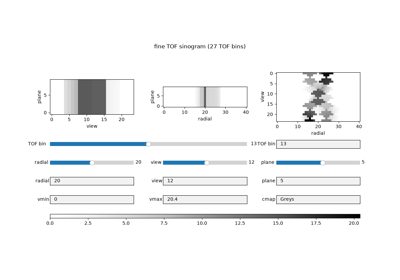
show_tof_bins(ax: Axes3D, tof_parameters: TOFParameters, views: int | Array | None = None, plane: int = 0, show_endpoints: bool = True, bin_cmap: str = 'seismic', show_bin_labels: bool = False, label_fontsize: float = 8.0, lw: float = 2.0, show_colorbar: bool = False) → None[source]¶

Visualise the TOF bin grid for the specified sinogram views and plane.

Each LOR is drawn as a sequence of coloured line segments – one per TOF bin – directly along the LOR (“zebra” style). Bin colour runs from blue (bin 0, xstart side) to red (bin N-1, xend side) via bin_cmap. Bins whose extent falls completely outside the physical LOR (i.e. beyond the detector positions) are silently skipped, so short edge LORs naturally show fewer coloured segments than central ones.

Parameters:

ax (Axes3D) – 3-D matplotlib axes to draw on. The caller is responsible for creating the figure and axes.
tof_parameters (TOFParameters) – TOF bin geometry (number of bins, bin width, centre offset).
views (int, array-like, or None) –
Sinogram view index / indices to draw.
- int – draw only that view.
- array-like – draw those specific views.
- None (default) – draw the single middle view (num_views // 2).
plane (int) – Sinogram plane index (axial ring pair). Default 0.
show_endpoints (bool) – Call show_lor_endpoints() to annotate detector positions. Default True.
bin_cmap (str) – Matplotlib colourmap for the bin segments. Default "seismic".
show_bin_labels (bool) – Annotate the bin numbers on the central LOR of the drawn set. Default False (useful only for scanners with few LORs).
label_fontsize (float) – Font size for bin labels when show_bin_labels=True.
lw (float) – Line width of the coloured bin segments. Default 2.0.
show_colorbar (bool) – Add a colorbar mapping bin index to colour. Default False.

Return type:

None

Examples

show_views(ax: Axes, views: Array, planes: Array, lw: float = 0.2, **kwargs) → None[source]¶

Show all LORs for the given views and planes.

Parameters:

ax (plt.Axes) – A 3D matplotlib axes.
views (Array) – Integer array of view indices to display.
planes (Array) – Integer array of plane indices to display.
lw (float, optional) – Line width, by default 0.2.

Return type:

None

Examples

property sinogram_order: SinogramSpatialAxisOrder¶: the order of the sinogram axes

property span: int | None¶: axial compression factor (1 = no compression; None for GE layout)

property spatial_sinogram_shape: tuple[int, ...]¶: the shape of the sinogram in spatial order

property start_in_ring_index: Array¶: start index within ring for all views - shape (num_views, num_rad)

property start_plane_index: Array¶: start ring index for all planes (only defined for single-ring-pair planes)

property start_plane_z: Array¶: start z-coordinate for all planes (averaged over constituent ring pairs for span > 1)

property view0_shift: int¶: detector-anchor shift m of the views (view 0’s central bin connects ((0 + m) mod N, (N/2 + m) mod N))

property view_axis_num: int¶: the axis number of the view axis

property view_direction: ViewDirection¶: direction in which the view index increases

property xp: ModuleType¶: array module to use for storing the LOR endpoints

property zig_zag_order: SinogramZigZagOrder¶: the zig-zag ordering convention for in-ring detector pairs

class parallelproj.pet_lors.SegmentOrder(*values)[source]¶

Bases: Enum

Order in which the signed oblique segments are laid out in a Michelogram.

Segment 0 always comes first; the two conventions differ only in whether the positive or the negative member of each \(\pm k\) pair precedes the other. This is a pure permutation of the sinogram planes – the number of planes, their multiplicities and the segment numbering (Michelogram.ring_diff_to_segment()) are unaffected.

Examples

NEGATIVE_FIRST = 2¶

Segments ordered 0, -1, +1, -2, +2, ....

Examples

POSITIVE_FIRST = 1¶

Segments ordered 0, +1, -1, +2, -2, ... (default).

Examples

classmethod __getitem__(name)¶

Return the member matching name.

Examples

class parallelproj.pet_lors.SinogramAxialCompressionOperator(lor_descriptor: RegularPolygonPETLORDescriptor, target_span: int | None = None, mode: str = 'sum', num_tof_bins: int | None = None, target_layout: MichelogramLayout = MichelogramLayout.STANDARD, target_segment_order: SegmentOrder = SegmentOrder.POSITIVE_FIRST)[source]¶

Bases: LinearOperator

Linear operator that axially compresses a span-1 PET sinogram to a higher odd span (or GE).

The output layout is chosen with target_layout: a STANDARD higher odd span (default) or the GE layout (target_layout=MichelogramLayout.GE, which ignores target_span). In both cases every span-1 ring pair is assigned to an output plane by the target Michelogram. A useful consequence: the mode="average" adjoint distributes a compressed sinogram back onto the span-1 grid while preserving counts – e.g. to un-combine a GE sinogram into span-1 (and then, say, mash it with SinogramMashingOperator).

For an input RegularPolygonPETLORDescriptor with span=1 and a target odd span \(S\), every span-1 ring pair \((s, e)\) is assigned to an output bin \((\text{segment}, \text{axial midpoint})\) where

segment is determined by the ring difference \(rd = e - s\) under target span \(S\) (see Michelogram.ring_diff_to_segment()),
axial midpoint is \(s + e\) (an integer equal to twice the actual midpoint).

All span-1 ring pairs sharing the same \((\text{segment}, s + e)\) collapse into a single output plane.

Two reduction modes are supported:

mode="sum" (default). The output plane is the sum of the contributing input planes:

\[y_n \;=\; \sum_{p_1 \in \mathcal{G}(n)} x_{p_1} \qquad \left(G^T y\right)_{p_1} \;=\; y_{\,\tau(p_1)}\,.\]

This is the natural reduction for counts-like sinograms – emission data, measured counts, randoms, etc. – which add when ring pairs are grouped together.
mode="average". The output plane is the mean of the contributing input planes:

\[y_n \;=\; \frac{1}{m_n} \sum_{p_1 \in \mathcal{G}(n)} x_{p_1} \qquad \left(G_{\rm avg}^T y\right)_{p_1} \;=\; \frac{y_{\,\tau(p_1)}}{m_{\,\tau(p_1)}}\,.\]

This is the natural reduction for multiplicative-factor sinograms – attenuation factors, sensitivity / normalisation factors, geometric efficiency – which should average rather than sum when ring pairs are grouped together.

In both expressions, \(\mathcal{G}(n)\) is the set of input plane indices mapped to output plane \(n\), \(m_n = |\mathcal{G}(n)|\) is the plane multiplicity, and \(\tau(p_1)\) is the output plane index for input plane \(p_1\).

Output plane ordering matches that of RegularPolygonPETLORDescriptor constructed with the same scanner, radial_trim, max_ring_difference, and sinogram_order but with span=target_span. That companion descriptor is exposed as out_lor_descriptor for visualization (e.g. show_michelogram, show_segment_lors) or for composing the operator with a span-\(S\) projector.

The closed-form operator 2-norms are

\[\|G_{\rm sum}\|_2 = \sqrt{\max_n m_n}\,, \qquad \|G_{\rm avg}\|_2 = 1 / \sqrt{\min_n m_n}\,,\]

derived from \(G_{\rm sum} G_{\rm sum}^T = \operatorname{diag}(m_n)\) and \(G_{\rm avg} G_{\rm avg}^T = \operatorname{diag}(1/m_n)\). norm() returns these directly without power iteration.

Parameters:

lor_descriptor (RegularPolygonPETLORDescriptor) – A span=1 LOR descriptor whose sinogram is to be compressed.
target_span (int or None) – Odd integer >= 1 giving the target axial compression (STANDARD layout). 1 is accepted and yields an identity-like operator (each input plane maps to a single output plane in the same span-1 order). Ignored (and may be None) when target_layout is MichelogramLayout.GE.
mode ({"sum", "average"}, optional) – Reduction mode. "sum" (default) is appropriate for counts-like sinograms; "average" is appropriate for multiplicative-factor sinograms such as attenuation or sensitivity factors. "average" is also the mode whose adjoint distributes a compressed sinogram back to span-1 while preserving counts (e.g. to un-combine a GE sinogram).
num_tof_bins (int or None, optional) – If None (default), the operator acts on the 3D spatial sinogram with shape RegularPolygonPETLORDescriptor.spatial_sinogram_shape. If a positive integer, the operator acts on a 4D TOF sinogram whose trailing axis (size num_tof_bins) is the TOF axis and is passed through unchanged.
target_layout (MichelogramLayout, optional) – Axial layout of the output sinogram. STANDARD (default) uses target_span; GE compresses the span-1 input to the GE layout (target_span is ignored). The GE target requires a span-1 input.
target_segment_order (SegmentOrder, optional) – Segment ordering of the output sinogram, by default SegmentOrder.POSITIVE_FIRST. See SegmentOrder.

Examples

>>> import array_api_compat.numpy as xp
>>> import parallelproj.pet_scanners as pps
>>> import parallelproj.pet_lors as ppl
>>> scanner = pps.RegularPolygonPETScannerGeometry(
...     xp, "cpu", radius=65.0, num_sides=12, num_lor_endpoints_per_side=4,
...     lor_spacing=4.0, ring_positions=xp.asarray([0.0, 1.0, 2.0]),
...     symmetry_axis=2,
... )
>>> lor_s1 = ppl.RegularPolygonPETLORDescriptor(
...     scanner, ppl.Michelogram(scanner.num_rings, 2, span=1), radial_trim=1,
... )
>>> comp = ppl.SinogramAxialCompressionOperator(lor_s1, target_span=3)
>>> comp.in_shape, comp.out_shape
((..., ..., 9), (..., ..., 7))
>>> comp.adjointness_test(xp, "cpu")
True

Examples

property H: AdjointLinearOperator¶: adjoint operator \(A^H\)

__call__(x: Array) → Array¶

alias to apply(x)

Examples

Parameters:: x (Array)
Return type:: Array

adjoint(y: Array) → Array¶

(scaled) adjoint step \(x = \overline{\alpha} A^H y\)

Parameters:: y (Array)
Return type:: Array

Examples

adjointness_test(xp: ModuleType | None = None, dev: str | None = None, verbose: bool = False, iscomplex: bool = False, dtype: type | None = None, **kwargs) → bool¶

test whether the adjoint is correctly implemented

Parameters:

xp (ModuleType, optional) – array module to use. Defaults to the operator’s own namespace (self.xp) when it exposes one; otherwise must be given.
dev (str, optional) – device (cpu or cuda). Defaults to the operator’s own device (self.dev) when it exposes one, else the default device.
verbose (bool, optional) – verbose output
iscomplex (bool, optional) – use complex arrays
dtype (type | None, optional) – data type of the arrays
**kwargs (dict) – passed to np.isclose

Returns:

whether the adjoint is correctly implemented

Return type:

bool

Examples

apply(x: Array) → Array¶

(scaled) forward step \(y = \alpha A x\)

Parameters:: x (Array)
Return type:: Array

Examples

property in_shape: tuple[int, ...]¶: Spatial sinogram shape of the span-1 input, optionally with a trailing TOF axis.

property lor_descriptor: RegularPolygonPETLORDescriptor¶: The input (span-1) LOR descriptor.

property max_plane_multiplicity: int¶: Largest plane multiplicity (\(\|G\|_2^2\)).

property mode: str¶: Reduction mode, either "sum" or "average".

norm(xp: ModuleType, dev: str, num_iter: int = 30, iscomplex: bool = False, verbose: bool = False) → float[source]¶

Operator 2-norm in closed form.

Because each input plane belongs to exactly one output plane,

mode="sum": \(G G^T = \operatorname{diag}(m_n)\) and therefore \(\|G\|_2 = \sqrt{\max_n m_n}\).
mode="average": \(G_{\rm avg} G_{\rm avg}^T = \operatorname{diag}(1/m_n)\) and therefore \(\|G_{\rm avg}\|_2 = 1 / \sqrt{\min_n m_n}\).

Both norms are independent of TOF, xp, and dev; the inherited signature is retained for compatibility with LinearOperator.norm but its arguments (xp, dev, num_iter, iscomplex, verbose) are ignored.

Examples

Parameters:

xp (ModuleType)
dev (str)
num_iter (int)
iscomplex (bool)
verbose (bool)

Return type:

float

property num_planes_in: int¶: Number of span-1 input planes.

property num_planes_out: int¶: Number of span-\(S\) output planes.

property num_tof_bins: int | None¶: Number of TOF bins, or None for a non-TOF operator.

property out_lor_descriptor: RegularPolygonPETLORDescriptor¶: Auto-built companion descriptor whose plane ordering matches this operator’s output.

property out_shape: tuple[int, ...]¶: Spatial sinogram shape of the compressed output, optionally with a trailing TOF axis.

property plane_multiplicity: Array¶

Number of span-1 planes that collapse into each output plane.

Shape (num_planes_n,). Equals the diagonal of \(G G^T\).

property scale: float | complex¶: scalar factor applied to the linear operator

property target_layout: MichelogramLayout¶: Axial layout of the output sinogram (STANDARD or GE).

property target_plane_for_input_plane: Array¶

Output plane index for each span-1 input plane.

Shape (num_planes_1,). Useful for the closed-form check \((G^T G\,\mathbf{1})_{p_1} = m_{\,\tau(p_1)}\).

property target_span: int | None¶: Target span (odd, >= 1), or None for a GE-layout target.

class parallelproj.pet_lors.SinogramMashingOperator(lor_descriptor: RegularPolygonPETLORDescriptor, transaxial_factor: int = 1, axial_factor: int = 1, mode: str = 'sum', coarse_radial_trim: int | None = None, num_tof_bins: int | None = None)[source]¶

Bases: LinearOperator

Detector mashing for a span-1 regular-polygon PET sinogram.

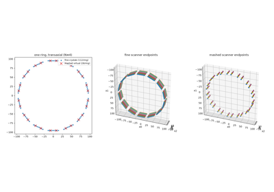
Groups neighbouring detectors into larger virtual detectors located at the average endpoint position, dramatically reducing the number of LORs.

transaxial_factor (\(N\)) groups \(N\) neighbouring crystals within each polygon side;
axial_factor (\(M\)) groups \(M\) neighbouring rings.

Because within-side averaging of uniformly spaced crystals (and of ring positions) again yields a regular polygon, the mashed geometry is itself a RegularPolygonPETScannerGeometry, exposed as coarse_scanner, with a matching span-1 coarse_lor_descriptor. A standard RegularPolygonPETProjector built on the latter projects directly along the mashed LORs (the fast, approximate forward model), while this operator composed with the fine projector is the exact mashed model.

The operator maps every fine sinogram bin to the coarse bin whose two virtual detectors contain the fine bin’s two endpoints, and

mode="sum" (default) sums the contributing fine bins – the natural reduction for counts-like data (emission, measured counts);
mode="average" takes their mean – appropriate for multiplicative factors (attenuation, normalisation) and matching a single coarse-geometry projector.

The adjoint scatters/broadcasts accordingly. Each fine bin maps to exactly one coarse bin, so \(G G^T = \operatorname{diag}(m_n)\) and the closed-form 2-norms are \(\|G_{\rm sum}\| = \sqrt{\max_n m_n}\), \(\|G_{\rm avg}\| = 1/\sqrt{\min_n m_n}\) with \(m_n\) the per-coarse-bin multiplicity; norm() returns these directly.

Constraints: the input descriptor must have span == 1, N must divide num_lor_endpoints_per_side and M must divide num_rings. GE-layout sinograms are mashed by composition: convert GE -> span-1 with the average-mode adjoint of a span-1 <-> GE SinogramAxialCompressionOperator, mash the span-1 sinogram with this operator, giving a pure span-1 coarse sinogram (see the detector-mashing example).

Parameters:

lor_descriptor (RegularPolygonPETLORDescriptor) – the fine (un-mashed) span-1 descriptor.
transaxial_factor (int, optional) – number of neighbouring within-side crystals to mash (N), default 1.
axial_factor (int, optional) – number of neighbouring rings to mash (M), default 1.
mode ({"sum", "average"}, optional) – reduction mode, default "sum".
coarse_radial_trim (int or None, optional) – radial trim of the coarse descriptor. None (default) derives it automatically from the fine->coarse mapping so that every coarse radial bin with at least one non-degenerate fine contributor is kept (no trimming-induced count loss) while no empty peripheral coarse radial bins remain. Pass an explicit non-negative integer to override this (a larger value trims additional radial bins and will discard the fine LORs that map into them).
num_tof_bins (int or None, optional) – if given, the operator acts on a 4D TOF sinogram whose trailing axis is passed through unchanged (an approximation: the averaged LOR direction differs slightly from the fine LORs).

Notes

TOF binning of the mashed LOR is approximate because the averaged endpoints define a slightly different LOR direction than the individual fine LORs.

Examples

property H: AdjointLinearOperator¶: adjoint operator \(A^H\)

__call__(x: Array) → Array¶

alias to apply(x)

Examples

Parameters:: x (Array)
Return type:: Array

adjoint(y: Array) → Array¶

(scaled) adjoint step \(x = \overline{\alpha} A^H y\)

Parameters:: y (Array)
Return type:: Array

Examples

adjointness_test(xp: ModuleType | None = None, dev: str | None = None, verbose: bool = False, iscomplex: bool = False, dtype: type | None = None, **kwargs) → bool¶

test whether the adjoint is correctly implemented

Parameters:

xp (ModuleType, optional) – array module to use. Defaults to the operator’s own namespace (self.xp) when it exposes one; otherwise must be given.
dev (str, optional) – device (cpu or cuda). Defaults to the operator’s own device (self.dev) when it exposes one, else the default device.
verbose (bool, optional) – verbose output
iscomplex (bool, optional) – use complex arrays
dtype (type | None, optional) – data type of the arrays
**kwargs (dict) – passed to np.isclose

Returns:

whether the adjoint is correctly implemented

Return type:

bool

Examples

apply(x: Array) → Array¶

(scaled) forward step \(y = \alpha A x\)

Parameters:: x (Array)
Return type:: Array

Examples

property axial_factor: int¶: number of rings mashed together (M).

property coarse_lor_descriptor: RegularPolygonPETLORDescriptor¶: the mashed (output) LOR descriptor.

property coarse_scanner¶: the mashed (averaged-endpoint) regular-polygon scanner geometry.

property in_shape: tuple[int, ...]¶: fine spatial sinogram shape (optionally with a trailing TOF axis).

property lor_descriptor: RegularPolygonPETLORDescriptor¶: the fine (input) LOR descriptor.

property mode: str¶: reduction mode, "sum" or "average".

norm(xp: ModuleType | None = None, dev: str | None = None, num_iter: int = 30, iscomplex: bool = False, verbose: bool = False) → float[source]¶

Closed-form operator 2-norm (arguments accepted but ignored).

mode="sum" -> sqrt(max multiplicity); mode="average" -> 1 / sqrt(min multiplicity).

Examples

Parameters:

xp (ModuleType | None)
dev (str | None)
num_iter (int)
iscomplex (bool)
verbose (bool)

Return type:

float

property num_tof_bins: int | None¶: number of TOF bins, or None for a non-TOF operator.

property out_shape: tuple[int, ...]¶: coarse spatial sinogram shape (optionally with a trailing TOF axis).

property scale: float | complex¶: scalar factor applied to the linear operator

property transaxial_factor: int¶: number of within-side crystals mashed together (N).

class parallelproj.pet_lors.SinogramSegmentSelectionOperator(lor_descriptor: RegularPolygonPETLORDescriptor, segments: Sequence[int], num_tof_bins: int | None = None)[source]¶

Bases: LinearOperator

Select a subset of Michelogram segments from a sinogram.

Given a (full) RegularPolygonPETLORDescriptor and a list of segments to keep, this operator

builds a companion restricted_lor_descriptor – identical to the input descriptor but with the segment-restricted Michelogram (Michelogram.select_segments()) – which you use to build the projector that produces/consumes the restricted sinogram directly;
as a LinearOperator, forward-gathers the selected planes of a full sinogram into the restricted one, and its adjoint scatters a restricted sinogram back into a zero-filled full sinogram.

The mapping only touches the plane axis (lor_descriptor.plane_axis_num), so both non-TOF (..., plane, ...) and TOF (..., plane, ..., tof) sinograms are supported (pass num_tof_bins). Because it is a pure plane selection (each kept plane maps to exactly one distinct output plane), forward and adjoint are exact transposes and \(\|G\|_2 = 1\).

Parameters:

lor_descriptor (RegularPolygonPETLORDescriptor) – the full LOR descriptor whose sinogram is the operator input.
segments (Sequence[int]) – signed segment numbers to keep (order/duplicates ignored; ordering of the restricted planes follows the michelogram’s segment_order).
num_tof_bins (int, optional) – if given, the sinograms carry a trailing TOF axis of this length; None (default) for non-TOF sinograms.

Example

>>> import array_api_compat.numpy as xp
>>> import parallelproj.pet_scanners as pps
>>> import parallelproj.pet_lors as ppl
>>> scanner = pps.RegularPolygonPETScannerGeometry(
...     xp, "cpu", radius=65.0, num_sides=4, num_lor_endpoints_per_side=2,
...     lor_spacing=4.0, ring_positions=xp.asarray([0.0, 1.0, 2.0]),
...     symmetry_axis=2)
>>> full = ppl.RegularPolygonPETLORDescriptor(
...     scanner, ppl.Michelogram(scanner.num_rings, 2, span=1))
>>> sel = ppl.SinogramSegmentSelectionOperator(full, segments=[0, -1, 1])
>>> sel.restricted_lor_descriptor.num_planes <= full.num_planes
True

Examples

property H: AdjointLinearOperator¶: adjoint operator \(A^H\)

__call__(x: Array) → Array¶

alias to apply(x)

Examples

Parameters:: x (Array)
Return type:: Array

adjoint(y: Array) → Array¶

(scaled) adjoint step \(x = \overline{\alpha} A^H y\)

Parameters:: y (Array)
Return type:: Array

Examples

adjointness_test(xp: ModuleType | None = None, dev: str | None = None, verbose: bool = False, iscomplex: bool = False, dtype: type | None = None, **kwargs) → bool¶

test whether the adjoint is correctly implemented

Parameters:

xp (ModuleType, optional) – array module to use. Defaults to the operator’s own namespace (self.xp) when it exposes one; otherwise must be given.
dev (str, optional) – device (cpu or cuda). Defaults to the operator’s own device (self.dev) when it exposes one, else the default device.
verbose (bool, optional) – verbose output
iscomplex (bool, optional) – use complex arrays
dtype (type | None, optional) – data type of the arrays
**kwargs (dict) – passed to np.isclose

Returns:

whether the adjoint is correctly implemented

Return type:

bool

Examples

apply(x: Array) → Array¶

(scaled) forward step \(y = \alpha A x\)

Parameters:: x (Array)
Return type:: Array

Examples

property in_shape: tuple[int, ...]¶: Spatial sinogram shape of the full input, optionally with a trailing TOF axis.

property lor_descriptor: RegularPolygonPETLORDescriptor¶: The full (input) LOR descriptor.

norm(xp: ModuleType, dev: str, num_iter: int = 30, iscomplex: bool = False, verbose: bool = False) → float[source]¶

Operator 2-norm in closed form.

Each kept plane maps to exactly one distinct output plane, so the rows of the selection matrix are orthonormal, \(G G^T = I\) and \(\|G\|_2 = 1\). The inherited signature is kept for API compatibility; its arguments are ignored.

Examples

Parameters:

xp (ModuleType)
dev (str)
num_iter (int)
iscomplex (bool)
verbose (bool)

Return type:

float

property num_planes_in: int¶: Number of planes in the full input sinogram.

property num_planes_out: int¶: Number of planes in the segment-restricted output sinogram.

property num_tof_bins: int | None¶: Number of TOF bins, or None for non-TOF sinograms.

property out_shape: tuple[int, ...]¶: Spatial sinogram shape of the segment-restricted output, optionally with a trailing TOF axis.

property restricted_lor_descriptor: RegularPolygonPETLORDescriptor¶: Companion descriptor with the segment-restricted Michelogram; use it to build the projector for the restricted sinogram.

property scale: float | complex¶: scalar factor applied to the linear operator

property segments: tuple[int, ...]¶: Kept segments, in the michelogram’s segment_order.

class parallelproj.pet_lors.SinogramSpatialAxisOrder(*values)[source]¶

Bases: Enum

order of spatial axis in a sinogram R (radial), V (view), P (plane)

Examples

Convergence comparison: SGD vs SVRG with logcosh regularization

PDHG and SPDHG for PET reconstruction with a directional TV prior

TOF vs non-TOF: variance reduction in a uniform cylinder

Convergence comparison: SGD vs SVRG with regularization (sinogram and listmode)

Penalised transmission reconstruction (MAPTR) with an edge-preserving prior

PRV = 5¶

[plane,radial,view]

Examples

PVR = 6¶

[plane,view,radial]

Examples

RPV = 2¶

[radial,plane,view]

Examples

RVP = 1¶

[radial,view,plane]

Examples

Convergence comparison: SGD vs SVRG with logcosh regularization

PDHG and SPDHG for PET reconstruction with a directional TV prior

TOF vs non-TOF: variance reduction in a uniform cylinder

Convergence comparison: SGD vs SVRG with regularization (sinogram and listmode)

PDHG and LM-SPDHG to optimize the Poisson logL and total variation

Transmission reconstruction: MLTR, SPS and L-BFGS-B

Accelerating MLTR with ordered subsets (OS-MLTR) and SVRG

Penalised transmission reconstruction (MAPTR) with an edge-preserving prior

Joint activity and attenuation reconstruction (MLAA) for TOF PET

VPR = 4¶

[view,plane,radial]

Examples

VRP = 3¶

[view,radial,plane]

Examples

classmethod __getitem__(name)¶

Return the member matching name.

Examples

class parallelproj.pet_lors.SinogramZigZagOrder(*values)[source]¶

Bases: Enum

Zig-zag ordering of in-ring detector pairs for each sinogram view.

For a scanner with \(n\) detector endpoints per ring and view index 0, the two variants differ in which detector (start or end) steps first as the radial bin index increases from the central LOR outward.

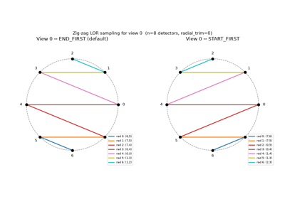
END_FIRST: The end detector steps first for each new radial pair. Pairs (start, end) at view 0: (0,n-1), (0,n-2), (1,n-2), (1,n-3), …
START_FIRST: The start detector steps first for each new radial pair. Pairs (start, end) at view 0: (0,n-1), (1,n-1), (1,n-2), (2,n-2), …

Examples

END_FIRST = 1¶

End crystal steps first (default, historically used convention).

Examples

START_FIRST = 2¶

Start crystal steps first.

Examples

classmethod __getitem__(name)¶

Return the member matching name.

Examples

class parallelproj.pet_lors.TOFBinMashingOperator(tof_parameters: TOFParameters, non_tof_data_shape: tuple[int, ...], mashing_factor: int = 1, mode: str = 'sum')[source]¶

Bases: LinearOperator

Linear operator that mashes (groups) neighbouring TOF bins.

Groups every mashing_factor (\(G\)) consecutive TOF bins of a TOF-binned data array into a single coarse bin. The reduction acts only on the trailing (TOF) axis; all leading (non-TOF) axes – e.g. the spatial sinogram axes, or listmode/block indices – are passed through unchanged. The operator is therefore geometry-agnostic: it works on any array whose last axis is the TOF axis (a plain length-num_tofbins vector included).

With \(G\) dividing the number of fine TOF bins, the fine bin index \(t\) maps to coarse bin \(t // G\), i.e. coarse bin \(c\) collects the fine bins \(\{cG, cG+1, \dots, cG+G-1\}\).

Two reduction modes are supported:

mode="sum" (default) – the coarse bin is the sum of its \(G\) fine bins:

\[y_c \;=\; \sum_{g=0}^{G-1} x_{\,cG+g} \qquad \left(A^T y\right)_t \;=\; y_{\,t // G}\,.\]

This is the natural reduction for counts-like TOF data. Because a TOF-bin weight is a Gaussian integrated over the bin’s extent and integrals over adjacent bins add exactly to the integral over their union, sum-mashing a TOF forward projection is (up to the num_sigmas truncation) identical to projecting directly onto the coarse TOF grid described by coarse_tof_parameters.
mode="average" – the coarse bin is the mean of its \(G\) fine bins:

\[y_c \;=\; \frac{1}{G} \sum_{g=0}^{G-1} x_{\,cG+g} \qquad \left(A_{\rm avg}^T y\right)_t \;=\; \frac{y_{\,t // G}}{G}\,.\]

The closed-form operator 2-norms follow from \(A A^T = G\,I\) (sum) and \(A_{\rm avg} A_{\rm avg}^T = (1/G)\,I\):

\[\|A_{\rm sum}\|_2 = \sqrt{G}\,, \qquad \|A_{\rm avg}\|_2 = 1 / \sqrt{G}\,.\]

norm() returns these directly without power iteration.

Parameters:

tof_parameters (TOFParameters) – TOF parameters of the fine (input) data. num_tofbins sets the fine TOF axis length; the mashed parameters are exposed as coarse_tof_parameters.
non_tof_data_shape (tuple of int) – Shape of the leading (non-TOF) axes. For a standard TOF sinogram pass lor_descriptor.spatial_sinogram_shape; pass () to act on a bare length-num_tofbins TOF vector.
mashing_factor (int, optional) – Number of neighbouring TOF bins grouped together (\(G\)), default 1 (identity along the TOF axis). Must divide tof_parameters.num_tofbins.
mode ({"sum", "average"}, optional) – Reduction mode, default "sum".

Notes

TOF-bin centring is a matter of convention and is not altered by this operator: for an odd num_tofbins the centre is the central bin (the LOR midpoint at TOF position 0); for an even num_tofbins the centre sits between the two central bins. Choose num_tofbins and mashing_factor so the coarse grid keeps the centring you want (e.g. an odd num_tofbins with an odd mashing_factor yields an odd coarse bin count and keeps a central bin).

Examples

>>> import array_api_compat.numpy as xp
>>> import parallelproj.tof as ppt
>>> import parallelproj.pet_lors as ppl
>>> tp = ppt.TOFParameters(num_tofbins=27, tofbin_width=25.0, sigma_tof=40.0)
>>> op = ppl.TOFBinMashingOperator(tp, (5, 8), mashing_factor=3)
>>> op.in_shape, op.out_shape
((5, 8, 27), (5, 8, 9))
>>> op.coarse_tof_parameters.num_tofbins, op.coarse_tof_parameters.tofbin_width
(9, 75.0)
>>> op.adjointness_test(xp, "cpu")
True

Examples

property H: AdjointLinearOperator¶: adjoint operator \(A^H\)

__call__(x: Array) → Array¶

alias to apply(x)

Examples

Parameters:: x (Array)
Return type:: Array

adjoint(y: Array) → Array¶

(scaled) adjoint step \(x = \overline{\alpha} A^H y\)

Parameters:: y (Array)
Return type:: Array

Examples

adjointness_test(xp: ModuleType | None = None, dev: str | None = None, verbose: bool = False, iscomplex: bool = False, dtype: type | None = None, **kwargs) → bool¶

test whether the adjoint is correctly implemented

Parameters:

xp (ModuleType, optional) – array module to use. Defaults to the operator’s own namespace (self.xp) when it exposes one; otherwise must be given.
dev (str, optional) – device (cpu or cuda). Defaults to the operator’s own device (self.dev) when it exposes one, else the default device.
verbose (bool, optional) – verbose output
iscomplex (bool, optional) – use complex arrays
dtype (type | None, optional) – data type of the arrays
**kwargs (dict) – passed to np.isclose

Returns:

whether the adjoint is correctly implemented

Return type:

bool

Examples

apply(x: Array) → Array¶

(scaled) forward step \(y = \alpha A x\)

Parameters:: x (Array)
Return type:: Array

Examples

property coarse_tof_parameters: TOFParameters¶

TOF parameters of the mashed grid.

num_tofbins is divided by mashing_factor and tofbin_width is multiplied by it; sigma_tof (the physical timing resolution), num_sigmas and tofcenter_offset are unchanged.

property in_shape: tuple[int, ...]¶: fine data shape non_tof_data_shape + (num_tofbins,).

property mashing_factor: int¶: number of neighbouring TOF bins mashed together (G).

property mode: str¶: reduction mode, "sum" or "average".

property non_tof_data_shape: tuple[int, ...]¶: shape of the leading (non-TOF) axes.

norm(xp: ModuleType | None = None, dev: str | None = None, num_iter: int = 30, iscomplex: bool = False, verbose: bool = False) → float[source]¶

Closed-form operator 2-norm (arguments accepted but ignored).

mode="sum" -> sqrt(mashing_factor); mode="average" -> 1 / sqrt(mashing_factor).

Examples

Parameters:

xp (ModuleType | None)
dev (str | None)
num_iter (int)
iscomplex (bool)
verbose (bool)

Return type:

float

property out_shape: tuple[int, ...]¶: mashed data shape non_tof_data_shape + (num_tofbins // G,).

property scale: float | complex¶: scalar factor applied to the linear operator

property tof_parameters: TOFParameters¶: the fine (input) TOF parameters.

class parallelproj.pet_lors.ViewDirection(*values)[source]¶

Bases: Enum

Direction in which the sinogram view index increases.

View 0 is always the central LOR through detectors (0, N/2); this enum only controls whether increasing the view index advances the detector pair in the + or - direction around the ring.

Examples