Regular polygon PET scanner geometry

This example shows how to create and visualize PET scanners where the LOR endpoints can be modeled as a stack of regular polygons.

import parallelproj.pet_scanners
import matplotlib.pyplot as plt

from parallelproj._examples_utils import suggest_array_backend_and_device

# To use a specific backend and/or device, replace the None arguments, e.g.:
#   xp, dev = suggest_array_backend_and_device(backend="numpy", dev="cpu") or by setting xp and dev manually
xp, dev = suggest_array_backend_and_device(None, None)

Using array API: array_api_compat.torch, device: cpu

Scanner coordinate system (symmetry_axis=2)

parallelproj labels the three world axes x0, x1, x2 rather than x, y, z. x0 is the left-most (first) axis of a 3-D image array (i.e. the axis you index first, img[i0, i1, i2]), x1 the second, and x2 the third.

For the common symmetry_axis=2 case the cylinder (axial) axis is x2. Picture yourself standing in front of the scanner, looking from -z to +z (into the bore):

• x0 (x) runs left to right,

• x1 (y) runs top to bottom (i.e. +x1 points down),

• x2 (z) runs away from you, into the scanner.

This right-handed convention is aligned with the DICOM/patient (LPS) axes for a head-first-supine patient, and it is why the 3-D plots below are drawn from that “in front of the scanner” viewpoint (ax.view_init(..., roll=180, vertical_axis="y")), so +x1 appears pointing downward.

Define four different PET scanners with different geometries

RegularPolygonPETScannerGeometry can be used to create the geometry of PET scanners where the LOR endpoints can be modeled as a stack of regular polygons.

Here we create four different PET scanners with different geometries. Note that symmetry_axis can be used to define which of the three axis is used as the cylinder (symmetry) axis.

scanner1 = parallelproj.pet_scanners.RegularPolygonPETScannerGeometry(
    xp,
    dev,
    radius=65.0,
    num_sides=12,
    num_lor_endpoints_per_side=8,
    lor_spacing=4.0,
    ring_positions=xp.linspace(-16, 16, 3, device=dev),
    symmetry_axis=2,
)

scanner2 = parallelproj.pet_scanners.RegularPolygonPETScannerGeometry(
    xp,
    dev,
    radius=65.0,
    num_sides=12,
    num_lor_endpoints_per_side=8,
    lor_spacing=4.0,
    ring_positions=xp.linspace(-16, 16, 3, device=dev),
    symmetry_axis=1,
)

scanner3 = parallelproj.pet_scanners.RegularPolygonPETScannerGeometry(
    xp,
    dev,
    radius=400.0,
    num_sides=32,
    num_lor_endpoints_per_side=16,
    lor_spacing=4.3,
    ring_positions=xp.linspace(-70, 70, 36, device=dev),
    symmetry_axis=2,
)

scanner4 = parallelproj.pet_scanners.RegularPolygonPETScannerGeometry(
    xp,
    dev,
    radius=400.0,
    num_sides=32,
    num_lor_endpoints_per_side=16,
    lor_spacing=4.3,
    ring_positions=xp.linspace(-70, 70, 36, device=dev),
    symmetry_axis=0,
)

Obtaining world coordinates of LOR endpoints

RegularPolygonPETScannerGeometry.get_lor_endpoints() can be used to obtain the world coordinates of the LOR endpoints

# get the world coordinates of the 4th LOR endpoint in the 1st "ring" (polygon)
# and the 5th LOR endpoint in the 2nd "ring" (polygon)
print("scanner1")
print(
    scanner1.get_lor_endpoints(
        xp.asarray([0, 1], device=dev), xp.asarray([3, 4], device=dev)
    )
)
print("scanner2")
print(
    scanner2.get_lor_endpoints(
        xp.asarray([0, 1], device=dev), xp.asarray([3, 4], device=dev)
    )
)

scanner1
tensor([[ -2., -65., -16.],
        [  2., -65.,   0.]])
scanner2
tensor([[-65., -16.,  -2.],
        [-65.,   0.,   2.]])

Visualize the defined LOR endpoints

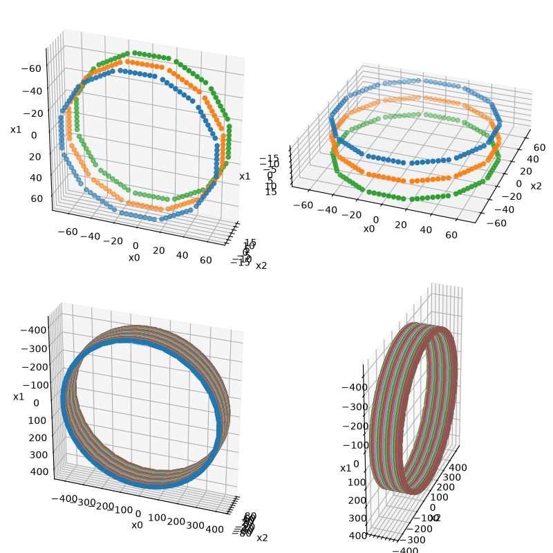
RegularPolygonPETScannerGeometry.show_lor_endpoints() can be used to visualize the defined LOR endpoints

fig = plt.figure(figsize=(8, 8), tight_layout=True)
ax1 = fig.add_subplot(221, projection="3d")
ax2 = fig.add_subplot(222, projection="3d")
ax3 = fig.add_subplot(223, projection="3d")
ax4 = fig.add_subplot(224, projection="3d")
for ax in (ax1, ax2, ax3, ax4):
    ax.view_init(elev=-30, azim=160, roll=180, vertical_axis="y")
scanner1.show_lor_endpoints(ax1)
scanner2.show_lor_endpoints(ax2)
scanner3.show_lor_endpoints(ax3)
scanner4.show_lor_endpoints(ax4)
fig.show()

Defining an open PET scanner geometry

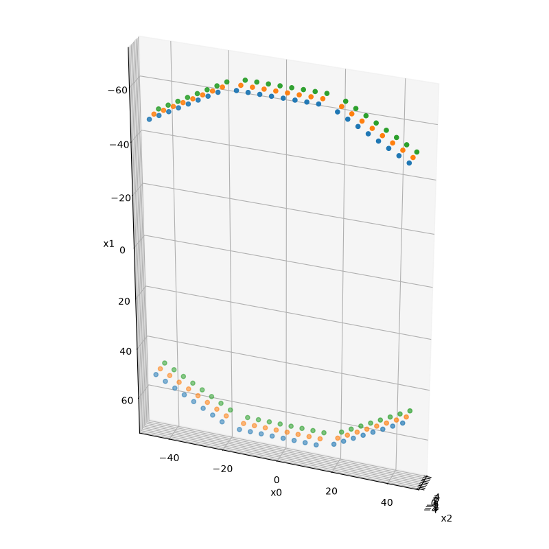
The phis argument can be used to manually define the azimuthal angles of the polygon “sides”. This can be used to create open PET scanner geometries. Here we create an open geometry with 6 sides and 3 rings corresponding to a full geometry using 12 sides where 6 sides were removed.

open_scanner = parallelproj.pet_scanners.RegularPolygonPETScannerGeometry(
    xp,
    dev,
    radius=65.0,
    num_sides=6,
    num_lor_endpoints_per_side=8,
    lor_spacing=4.0,
    ring_positions=xp.linspace(-4, 4, 3),
    symmetry_axis=2,
    phis=(2 * xp.pi / 12) * xp.asarray([-1, 0, 1, 5, 6, 7], device=dev),
)

fig2 = plt.figure(figsize=(8, 8), tight_layout=True)
ax2a = fig2.add_subplot(111, projection="3d")
ax2a.view_init(elev=-30, azim=160, roll=180, vertical_axis="y")
open_scanner.show_lor_endpoints(ax2a)
fig2.show()

Endpoint ordering and phi0: all four combinations

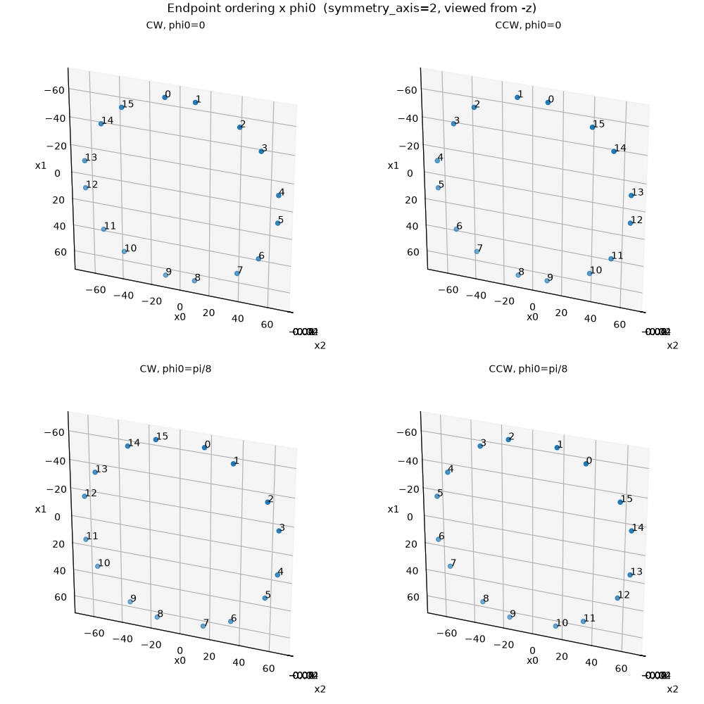
By default, endpoint indices increase clockwise when the ring is viewed from the negative symmetry-axis direction (for symmetry_axis=2: from -z toward +z, the default 3D view with +x right and +y down). Index 0 sits at the top (-y). RingEndpointOrdering lets you switch to counterclockwise ordering. The phi0 parameter rotates the starting angle of side 0 (in radians) as a right-hand rotation about the symmetry axis (positive phi0 moves side 0 toward +x); it is ignored when phis is supplied explicitly.

The 2x2 grid below shows all combinations of CW/CCW ordering with phi0=0 and phi0=pi/8 (half a polygon step for an 8-sided scanner).

import math

_RO = parallelproj.pet_scanners.RingEndpointOrdering

configs = [
    (_RO.CLOCKWISE, 0.0, "CW, phi0=0"),
    (_RO.COUNTERCLOCKWISE, 0.0, "CCW, phi0=0"),
    (_RO.CLOCKWISE, math.pi / 8, "CW, phi0=pi/8"),
    (_RO.COUNTERCLOCKWISE, math.pi / 8, "CCW, phi0=pi/8"),
]

fig3, axes = plt.subplots(
    2, 2, figsize=(10, 10), subplot_kw={"projection": "3d"}, layout="constrained"
)

for ax, (ordering, phi0, title) in zip(axes.flat, configs):
    scanner = parallelproj.pet_scanners.RegularPolygonPETScannerGeometry(
        xp,
        dev,
        radius=65.0,
        num_sides=8,
        num_lor_endpoints_per_side=2,
        lor_spacing=20.0,
        ring_positions=xp.asarray([0.0], device=dev),
        symmetry_axis=2,
        ring_endpoint_ordering=ordering,
        phi0=phi0,
    )
    ax.view_init(elev=-30, azim=160, roll=180, vertical_axis="y")
    scanner.show_lor_endpoints(ax, show_linear_index=True, annotation_fontsize=10)
    ax.set_title(title, fontsize="medium")

fig3.suptitle(
    "Endpoint ordering x phi0  (symmetry_axis=2, viewed from -z)", fontsize=12
)
fig3.show()

Non-uniform crystal spacing: subblock detector modules

The lor_endpoint_positions argument accepts a 1-D array of crystal positions (in mm, centred at 0) along each polygon side. This allows non-uniform layouts such as subblock detectors where crystals are grouped with a small intra-block pitch and a larger gap between blocks.

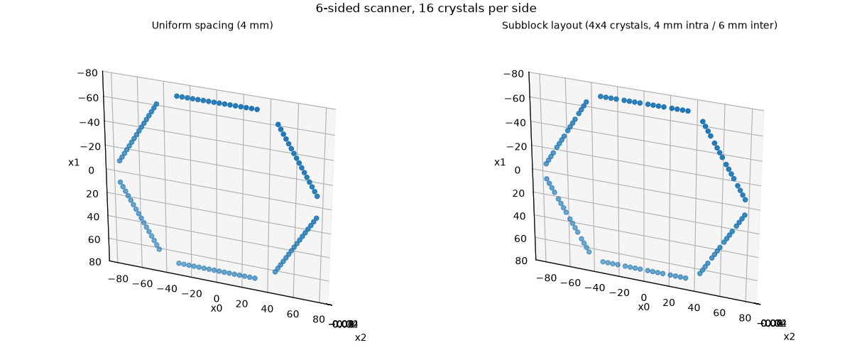
Here we build a 6-sided scanner with 16 crystals per side arranged in 4 subblocks of 4 crystals:

• intra-subblock pitch: 4 mm

• extra gap between adjacent subblocks: 2 mm (so the inter-subblock crystal distance is 4 + 2 = 6 mm)

For radial sinogram symmetry the position array must be anti-symmetric about 0 (pos[i] == -pos[N-1-i]), which is the case here.

Positions along each side (mm):

subblock 1       subblock 2       subblock 3       subblock 4
-33 -29 -25 -21  -15 -11  -7  -3  +3  +7 +11 +15  +21 +25 +29 +33

import numpy as np

num_subblocks = 4
n_per_subblock = 4
pitch = 4.0  # mm within a subblock
extra_gap = 2.0  # mm added between adjacent subblocks

# Within-subblock offsets centred at 0
sub_offsets = pitch * (np.arange(n_per_subblock) - (n_per_subblock - 1) / 2.0)
# = [-6, -2, +2, +6] mm

# Subblock centres: adjacent subblock centres are separated by
# (subblock span) + (intra-subblock pitch + extra gap)
subblock_span = (n_per_subblock - 1) * pitch  # 12 mm
centre_to_centre = subblock_span + pitch + extra_gap  # 18 mm

sub_centers = centre_to_centre * (np.arange(num_subblocks) - (num_subblocks - 1) / 2.0)
# = [-27, -9, +9, +27] mm

lor_endpoint_positions = xp.asarray(
    (sub_centers[:, None] + sub_offsets[None, :]).ravel(),
    dtype=xp.float32,
    device=dev,
)
# = [-33, -29, -25, -21, -15, -11, -7, -3, +3, +7, +11, +15, +21, +25, +29, +33]

scanner5 = parallelproj.pet_scanners.RegularPolygonPETScannerGeometry(
    xp,
    dev,
    radius=70.0,
    num_sides=6,
    ring_positions=xp.asarray([0.0], dtype=xp.float32, device=dev),
    symmetry_axis=2,
    lor_endpoint_positions=lor_endpoint_positions,
)

Visualize the subblock scanner and compare endpoint positions with uniform spacing

fig5, (ax5a, ax5b) = plt.subplots(
    1, 2, figsize=(12, 5), subplot_kw={"projection": "3d"}, layout="constrained"
)

# uniform reference (same N and pitch — no gap)
scanner5_uniform = parallelproj.pet_scanners.RegularPolygonPETScannerGeometry(
    xp,
    dev,
    radius=70.0,
    num_sides=6,
    num_lor_endpoints_per_side=16,
    lor_spacing=pitch,
    ring_positions=xp.asarray([0.0], dtype=xp.float32, device=dev),
    symmetry_axis=2,
)

for ax in (ax5a, ax5b):
    ax.view_init(elev=-30, azim=160, roll=180, vertical_axis="y")

scanner5_uniform.show_lor_endpoints(ax5a)
ax5a.set_title("Uniform spacing (4 mm)", fontsize="medium")

scanner5.show_lor_endpoints(ax5b)
ax5b.set_title(
    "Subblock layout (4x4 crystals, 4 mm intra / 6 mm inter)", fontsize="medium"
)

fig5.suptitle("6-sided scanner, 16 crystals per side", fontsize=12)
fig5.show()