TOF-bin mashing: fewer, wider time-of-flight bins

TOF mashing groups neighbouring time-of-flight (TOF) bins into fewer, wider bins. This shrinks the TOF axis of a sinogram (less memory, faster reconstruction) at the cost of TOF resolution – completely independent of any detector / LOR mashing along the spatial axes.

TOFBinMashingOperator groups every mashing_factor (\(G\)) neighbouring TOF bins. It only touches the trailing (TOF) axis, so all leading axes (here the spatial sinogram axes) pass through unchanged:

• mode="sum" (default) – coarse bin = sum of its \(G\) fine bins. Use it for counts-like data. Because a TOF-bin weight is a Gaussian integrated over the bin, and integrals over adjacent bins add up exactly, sum-mashing a TOF forward projection is (up to the num_sigmas truncation) identical to projecting directly onto the coarse TOF grid.

• mode="average" – coarse bin = mean of its \(G\) fine bins. Use it for multiplicative factors.

The matching coarse TOF parameters (num_tofbins divided by \(G\), tofbin_width multiplied by it) are exposed as .coarse_tof_parameters so a projector can be pointed straight at the mashed grid.

import numpy as np
import matplotlib.pyplot as plt

import parallelproj.pet_scanners
import parallelproj.pet_lors
import parallelproj.projectors
import parallelproj.tof
from parallelproj.operators import CompositeLinearOperator
from parallelproj import to_numpy_array

from parallelproj._examples_utils import suggest_array_backend_and_device, show_vol_cuts

# To use a specific backend and/or device, replace the None arguments, e.g.:
#   xp, dev = suggest_array_backend_and_device(backend="numpy", dev="cpu")
xp, dev = suggest_array_backend_and_device(None, None)

# ``show_vol_cuts`` returns interactive widgets; keep references so their
# callbacks are not garbage-collected.
_keep = []


def _tof_first(sino):
    """Move the trailing TOF axis to the front: (radial, view, plane, TOF) ->
    (TOF, radial, view, plane), so ``show_vol_cuts`` puts a slider on the TOF
    bin and shows spatial (radial/view/plane) cuts for the selected bin."""
    return np.moveaxis(to_numpy_array(sino), -1, 0)


_SINO_LABELS = ("TOF bin", "radial", "view", "plane")

Using array API: array_api_compat.torch, device: cpu

A TOF-capable scanner, sinogram descriptor and projector

A small cylindrical scanner is enough to illustrate the TOF axis.

num_rings = 4
scanner = parallelproj.pet_scanners.RegularPolygonPETScannerGeometry(
    xp,
    dev,
    radius=100.0,
    num_sides=12,
    num_lor_endpoints_per_side=4,
    lor_spacing=4.0,
    ring_positions=xp.linspace(-6.0, 6.0, num_rings, device=dev),
    symmetry_axis=2,
)

lor_desc = parallelproj.pet_lors.RegularPolygonPETLORDescriptor(
    scanner,
    parallelproj.pet_lors.Michelogram(scanner.num_rings, max_ring_difference=1, span=1),
    radial_trim=3,
)

Fine TOF parameters: 27 bins. tofbin_width and sigma_tof are in mm (see TOFParameters for the ns -> mm conversion).

fine_tof = parallelproj.tof.TOFParameters(
    num_tofbins=27,
    tofbin_width=20.0,
    sigma_tof=30.0,
    num_sigmas=3.0,
)

A simple emission image and its fine, TOF-resolved forward projection.

img_shape = (40, 40, num_rings)
voxel_size = (4.0, 4.0, 4.0)

img = xp.zeros(img_shape, dtype=xp.float32, device=dev)
img[10:18, 18:30, :] = 1.0
img[24:30, 12:22, :] = 2.0

proj_fine = parallelproj.projectors.RegularPolygonPETProjector(
    lor_desc, img_shape, voxel_size
)
proj_fine.tof_parameters = fine_tof  # setting the parameters enables TOF

fine_sino = proj_fine(img)  # shape: spatial_sinogram_shape + (27,)
print(f"fine TOF sinogram shape : {tuple(fine_sino.shape)}")

fine TOF sinogram shape : (41, 24, 10, 27)

Mash the TOF bins

Group every G=3 neighbouring TOF bins (27 -> 9). mashing_factor must divide num_tofbins. Only the trailing TOF axis changes.

G = 3
tof_mash = parallelproj.pet_lors.TOFBinMashingOperator(
    fine_tof,
    lor_desc.spatial_sinogram_shape,
    mashing_factor=G,
    mode="sum",
)
print(tof_mash)
print(f"norm (sum mode)         : {tof_mash.norm():.4f}  (== sqrt({G}))")

coarse_tof = tof_mash.coarse_tof_parameters
print(
    f"coarse TOF parameters   : num_tofbins={coarse_tof.num_tofbins}, "
    f"tofbin_width={coarse_tof.tofbin_width} mm, sigma_tof={coarse_tof.sigma_tof} mm"
)

mashed_sino = tof_mash(fine_sino)  # shape: spatial_sinogram_shape + (9,)
print(f"mashed TOF sinogram     : {tuple(mashed_sino.shape)}")

TOFBinMashingOperator(mashing_factor=3, mode='sum', num_tofbins: 27 -> 9, non_tof_data_shape=(41, 24, 10))
norm (sum mode)         : 1.7321  (== sqrt(3))
coarse TOF parameters   : num_tofbins=9, tofbin_width=60.0 mm, sigma_tof=30.0 mm
mashed TOF sinogram     : (41, 24, 10, 9)

Scroll through the TOF sinograms

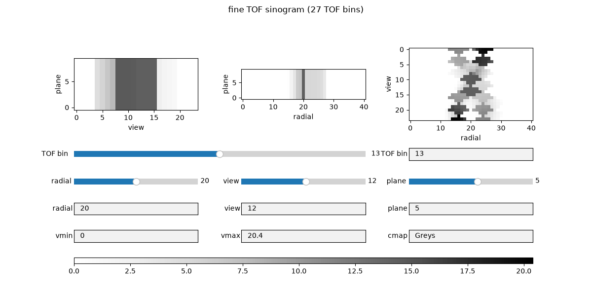
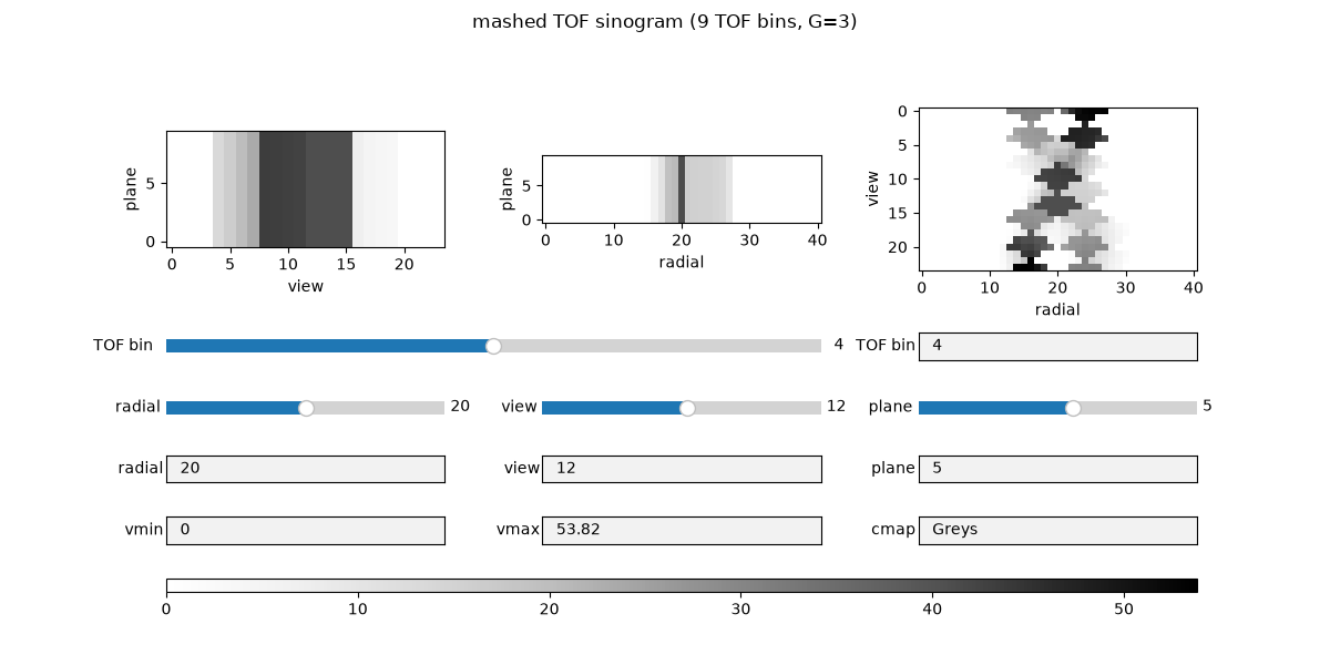
Both sinograms are 4-D (radial, view, plane, TOF). show_vol_cuts takes the TOF bin as the leading (slider) axis and shows the spatial cuts for the selected bin, so you can scroll through the TOF bins on the left and the spatial axes on the right. The mashed sinogram has 9 TOF bins instead of 27.

_keep.append(
    show_vol_cuts(
        _tof_first(fine_sino),
        axis_labels=_SINO_LABELS,
        fig_title=f"fine TOF sinogram ({fine_tof.num_tofbins} TOF bins)",
    )
)
_keep.append(
    show_vol_cuts(
        _tof_first(mashed_sino),
        axis_labels=_SINO_LABELS,
        fig_title=f"mashed TOF sinogram ({coarse_tof.num_tofbins} TOF bins, G={G})",
    )
)

• 
• 

TOF profile before and after mashing

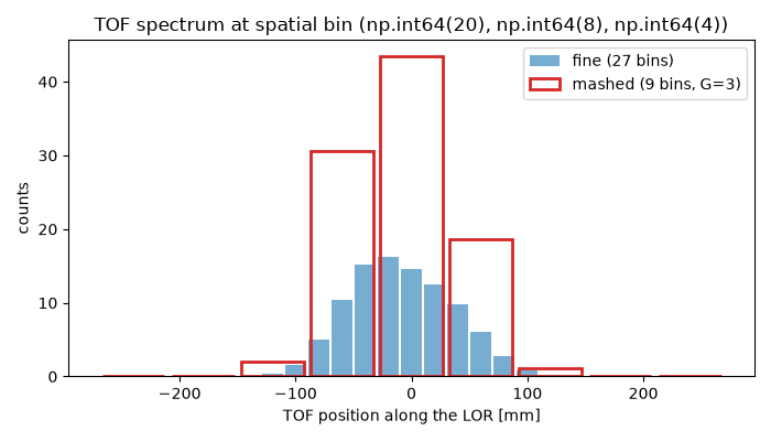
Pick the spatial sinogram bin with the most counts and plot its TOF spectrum. The 27 fine bins collapse into 9 wider bins whose heights are the sums of the three fine bins they cover; the total number of counts is preserved.

fine_np = to_numpy_array(fine_sino)
mashed_np = to_numpy_array(mashed_sino)

tof_axis = fine_sino.ndim - 1
spatial_counts = fine_np.sum(axis=tof_axis)
peak = np.unravel_index(np.argmax(spatial_counts), spatial_counts.shape)

fine_profile = fine_np[peak]  # (27,)
mashed_profile = mashed_np[peak]  # (9,)

# physical TOF-bin centres (mm), symmetric about 0
fine_centers = (np.arange(fine_tof.num_tofbins) - (fine_tof.num_tofbins - 1) / 2) * (
    fine_tof.tofbin_width
)
coarse_centers = (
    np.arange(coarse_tof.num_tofbins) - (coarse_tof.num_tofbins - 1) / 2
) * coarse_tof.tofbin_width

fig, ax = plt.subplots(1, 1, figsize=(7, 4), tight_layout=True)
ax.bar(
    fine_centers,
    fine_profile,
    width=fine_tof.tofbin_width * 0.9,
    color="tab:blue",
    alpha=0.6,
    label=f"fine ({fine_tof.num_tofbins} bins)",
)
ax.bar(
    coarse_centers,
    mashed_profile,
    width=coarse_tof.tofbin_width * 0.9,
    facecolor="none",
    edgecolor="tab:red",
    linewidth=2.0,
    label=f"mashed ({coarse_tof.num_tofbins} bins, G={G})",
)
ax.set_xlabel("TOF position along the LOR [mm]")
ax.set_ylabel("counts")
ax.set_title(f"TOF spectrum at spatial bin {peak}")
ax.legend()
fig.show()

Exactness of the sum-mashed forward model

For mode="sum", mashing the fine TOF projection is equivalent to projecting directly onto the coarse TOF grid (coarse_tof_parameters). We verify this by building a second projector on the same geometry but with the coarse TOF parameters.

proj_coarse = parallelproj.projectors.RegularPolygonPETProjector(
    lor_desc, img_shape, voxel_size
)
proj_coarse.tof_parameters = coarse_tof
coarse_sino_direct = proj_coarse(img)

rel_err = float(
    np.linalg.norm(mashed_np - to_numpy_array(coarse_sino_direct))
    / np.linalg.norm(to_numpy_array(coarse_sino_direct))
)
print(f"|| mash(P_fine x) - P_coarse x || / || P_coarse x || = {rel_err:.2e}")

# The directly-projected coarse TOF sinogram is (visually and numerically)
# identical to the mashed one above.
_keep.append(
    show_vol_cuts(
        _tof_first(coarse_sino_direct),
        axis_labels=_SINO_LABELS,
        fig_title=f"direct coarse-TOF projection ({coarse_tof.num_tofbins} TOF bins)",
    )
)

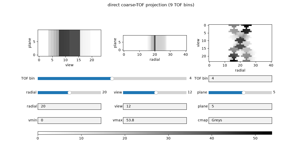
|| mash(P_fine x) - P_coarse x || / || P_coarse x || = 3.93e-04

Upsample the mashed sinogram back to the fine TOF grid

The adjoint maps a coarse TOF sinogram back onto the fine TOF grid. The two modes give two different upsamplings:

• the sum-mode adjoint replicates each coarse bin into its \(G\) fine bins. The summed counts are copied verbatim, so the values are ~ \(G\) times larger than the original fine sinogram (this is the genuine transpose used inside reconstruction, not a rescaled view of the data);

• the average-mode adjoint additionally divides by \(G\), spreading each coarse bin’s counts evenly over its fine bins. Each fine bin then holds the group mean, so the result is on the same scale as – and directly comparable to – the original fine TOF sinogram (a piecewise-constant approximation along the TOF axis).

So the average-mode adjoint is the one to use when the upsampled sinogram should be compared to the fine one.

Note

To upsample a coarse (mashed) sinogram back to the fine TOF grid, use the operator’s adjoint. The adjoint is not the inverse – mashing discards information, so tof_mash.adjoint(tof_mash(x)) != x. Choose the mode by what you want to keep: the mode="sum" adjoint replicates the coarse value into every fine bin (per-bin value preserved, total grows ~ G), while the mode="average" adjoint spreads it (divides by G; total counts preserved, per-bin value lowered and comparable to the fine data).

tof_mash_avg = parallelproj.pet_lors.TOFBinMashingOperator(
    fine_tof,
    lor_desc.spatial_sinogram_shape,
    mashing_factor=G,
    mode="average",
)

replicated = tof_mash.adjoint(mashed_sino)  # sum-mode adjoint: ~G x too large
upsampled = tof_mash_avg.adjoint(mashed_sino)  # average-mode adjoint: fine scale
assert tof_mash.adjointness_test(xp, dev, dtype=xp.float64)
assert tof_mash_avg.adjointness_test(xp, dev, dtype=xp.float64)

rel_up = float(
    np.linalg.norm(to_numpy_array(upsampled) - fine_np) / np.linalg.norm(fine_np)
)
print(
    f"upsampled shape         : {tuple(upsampled.shape)}  (back on the fine TOF grid)"
)
print(f"upsampled (avg-adjoint) vs fine, rel. difference = {rel_up:.2f}")

# The upsampled sinogram lives on the fine 27-bin TOF grid and matches the
# original fine sinogram up to the within-group TOF averaging.
_keep.append(
    show_vol_cuts(
        _tof_first(upsampled),
        axis_labels=_SINO_LABELS,
        fig_title=f"upsampled sinogram (avg-adjoint, {fine_tof.num_tofbins} TOF bins)",
    )
)

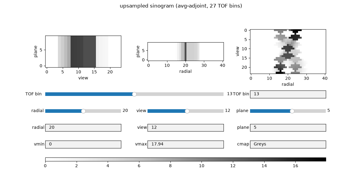
upsampled shape         : (41, 24, 10, 27)  (back on the fine TOF grid)
upsampled (avg-adjoint) vs fine, rel. difference = 0.32

Combine with geometric (detector) mashing

TOF-bin mashing composes with SinogramMashingOperator (which mashes the spatial LOR axes). Compress the TOF axis first, then mash the geometry; CompositeLinearOperator gives the combined operator (and its adjoint) for free. Note the spatial operator is told how many TOF bins remain after TOF mashing.

spatial_mash = parallelproj.pet_lors.SinogramMashingOperator(
    lor_desc,
    transaxial_factor=2,
    axial_factor=2,
    mode="sum",
    num_tof_bins=coarse_tof.num_tofbins,
)

full_mash = CompositeLinearOperator([spatial_mash, tof_mash])  # TOF first, then spatial
full_sino = full_mash(fine_sino)

n_in = int(np.prod(full_mash.in_shape))
n_out = int(np.prod(full_mash.out_shape))
print(f"combined mashing        : {full_mash.in_shape} -> {full_mash.out_shape}")
print(f"total data reduction    : {n_in / n_out:.1f}x")

combined mashing        : (41, 24, 10, 27) -> (21, 12, 4, 9)
total data reduction    : 29.3x

plt.show()