Exact vs. “safe epsilon” mode of the negative Poisson log-likelihood

NegPoissonLogL offers two evaluation modes:

1. exact=True evaluates the unmodified negative Poisson log-likelihood

   \[f(\bar{y}) = \sum_i \bar{y}_i - y_i \log \bar{y}_i .\]

   Bins with \(y_i = 0\) (virtual bins without geometric sensitivity, or active bins that measured zero counts) are handled exactly via their analytic values, so this mode requires \(\bar{y}_i > 0\) only in bins with counts (\(y_i > 0\)). If that requirement is violated, the function value is \(+\infty\) and the gradient \(-\infty\) – mathematically correct, but fatal for gradient-based iterative algorithms (and cupy / torch produce these infinities silently).

2. The default (“safe epsilon”) mode evaluates a shifted Poisson surrogate, where a tiny \(\varepsilon\) = rel_eps * mean(y) is added to both the measured and the expected data:

   \[f_\varepsilon(\bar{y}) = \sum_i (\bar{y}_i + \varepsilon) - (y_i + \varepsilon) \log(\bar{y}_i + \varepsilon), \qquad \nabla f_\varepsilon = \frac{\bar{y} - y}{\bar{y} + \varepsilon}.\]

   This is finite and smooth for any non-negative expectation, the per-bin minimiser remains exactly at \(\bar{y}_i = y_i\), and the gradient bias w.r.t. the exact log-likelihood is proportional to the residual (it vanishes at the fit).

When to use which? Use exact=True whenever you can rule out \(\bar{y}_i = 0\) in bins with counts – e.g. a strictly positive contamination (scatter + randoms) in all non-virtual bins, which is the common situation in practice. Keep the default whenever the expectation can reach zero in a bin with counts. The subtle danger is forward model mismatch: if the reconstruction model assigns exactly zero sensitivity to a bin that recorded a count (kernel truncation, geometric mismatch, float32 underflow of long tails), the exact mode blows up.

This example constructs precisely that situation: MLEM (in its EM-preconditioned gradient descent form) for \(y \sim \text{Poisson}(A x)\) where \(A\) is a 1D Gaussian convolution (GaussianFilterOperator) and the true image is a centered point source. The data are generated with the Gaussian kernel truncated at \(7\sigma\), while the reconstruction truncates the same kernel at \(4\sigma\) (scipy’s truncate kwarg). Counts recorded between \(4\sigma\) and \(7\sigma\) then fall in bins where the reconstruction model of the point source predicts exactly zero – and starting MLEM at the “correct” image (the true point source) immediately produces infinite gradients in exact mode, while the default mode runs unharmed.

import matplotlib.pyplot as plt
import numpy as np

import parallelproj.operators
from parallelproj import to_numpy_array
from parallelproj.functions import C2AffineObjective, NegPoissonLogL

from parallelproj._examples_utils import suggest_array_backend_and_device

# To use a specific backend and/or device, replace the None arguments, e.g.:
#   xp, dev = suggest_array_backend_and_device(backend="numpy", dev="cpu")
xp, dev = suggest_array_backend_and_device(None, None)

Using array API: array_api_compat.torch, device: cpu

1D Gaussian convolution forward models

Both models share the same Gaussian sigma; they differ only in where the kernel is truncated to exactly zero (scipy’s truncate kwarg, in units of sigma). The data model keeps the tails up to \(7\sigma\), the reconstruction model cuts them at \(4\sigma\).

n = 61  # number of pixels / bins
sig = 2.0  # Gaussian sigma in pixels
amp = 3e8  # amplitude (expected counts) of the point source

# forward model used to generate the data (truncation at 7 sigma)
A_data = parallelproj.operators.GaussianFilterOperator((n,), sigma=sig, truncate=7.0)
# forward model used for the reconstruction (truncation at 4 sigma)
A_rec = parallelproj.operators.GaussianFilterOperator((n,), sigma=sig, truncate=4.0)

Simulate Poisson data from a centered point source

x_true = xp.zeros(n, dtype=xp.float32, device=dev)
x_true[n // 2] = amp

exp_data = A_data(x_true)  # noise-free expectation (data model, 7 sigma)
exp_rec = A_rec(x_true)  # expectation of the recon model at the true image

np.random.seed(3)
y = xp.asarray(
    np.random.poisson(to_numpy_array(exp_data)), device=dev, dtype=xp.float32
)

# the MLEM / EM preconditioner denominator A^T 1 (= 1 for a normalised kernel)
sens = A_rec.adjoint(xp.ones(A_rec.out_shape, dtype=xp.float32, device=dev))

Expectation and counts profiles – the problem bins

The expectation of the true image under the reconstruction model is exactly zero beyond \(4\sigma\), but a few of those bins recorded counts (the data model extends to \(7\sigma\)). These are clearly visible in the zoomed panel.

problem = (exp_rec == 0) & (y > 0)
num_problem = int(xp.sum(xp.astype(problem, xp.int32)))
print(f"bins with y > 0 but expectation = 0 at the true image: {num_problem}")

i = np.arange(n)
y_np = to_numpy_array(y)
exp_data_np = to_numpy_array(exp_data)
exp_rec_np = to_numpy_array(exp_rec)

fig, ax = plt.subplots(1, 2, figsize=(11, 4.5), tight_layout=True)
for a in ax:
    a.plot(
        i,
        exp_data_np,
        "v",
        color="C0",
        ms=5,
        label=r"exp. $Ax_{true}$ (7$\sigma$)",
    )
    a.plot(
        i,
        exp_rec_np,
        "x",
        color="C1",
        ms=5,
        label=r"exp. $A'x_{true}$ (4$\sigma$)",
    )
    a.plot(i, y_np, ".", color="k", ms=6, label="measured counts $y$")
    a.set_xlabel("bin")
    a.grid(ls=":")
ax[0].set_title("expectation and counts profile")
ax[0].legend(loc="upper left")
ax[1].set_ylim(-0.05, 1.1)
ax[1].set_title("zoom: counts in bins with zero recon-model expectation")
fig.show()

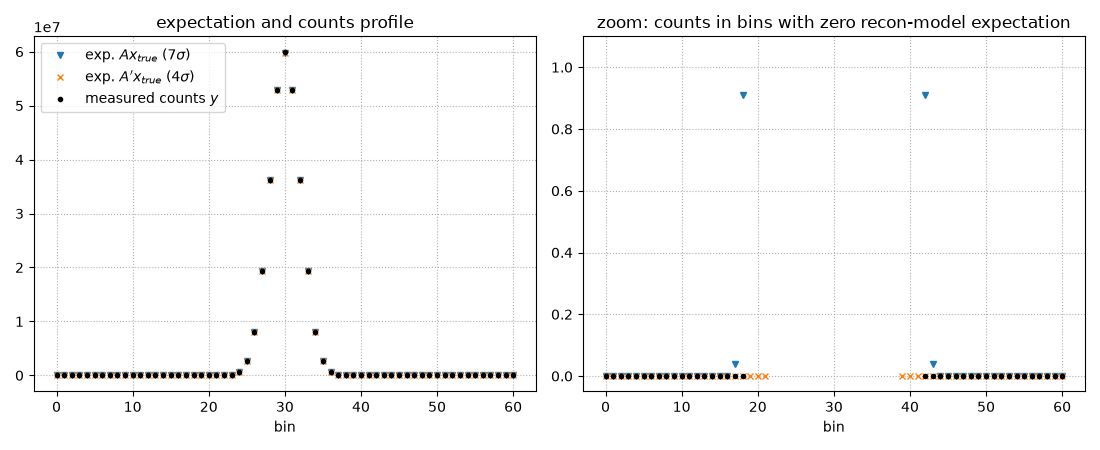
bins with y > 0 but expectation = 0 at the true image: 6

Exact mode: MLEM updates from the true image -> infinite gradients

We run MLEM in its EM-preconditioned gradient descent form

\[x^{(k+1)} = x^{(k)} - \frac{x^{(k)}}{A^T 1} \, \nabla f(x^{(k)})\]

starting at the true point source. At the problem bins the exact bin-space gradient is \(-\infty\); the backprojection spreads the infinities over the image, and from the second update on everything is nan. np.errstate only silences numpy’s warnings here – cupy / torch would produce the same result without any warning.

loss_exact = NegPoissonLogL(y, exact=True)
obj_exact = C2AffineObjective(loss_exact, A_rec)

x = x_true
for it in range(3):
    with np.errstate(divide="ignore", invalid="ignore"):
        grad_bin = loss_exact.gradient(A_rec(x))  # gradient in bin space
        grad_img = obj_exact.gradient(x)  # backprojected (image space)
        x = x - x / sens * grad_img  # EM-preconditioned GD step

    n_inf_bin = int(xp.sum(xp.astype(xp.isinf(grad_bin), xp.int32)))
    n_nonfin_img = int(xp.sum(xp.astype(~xp.isfinite(grad_img), xp.int32)))
    n_nonfin_x = int(xp.sum(xp.astype(~xp.isfinite(x), xp.int32)))
    print(
        f"exact mode, update {it + 1}: "
        f"{n_inf_bin:2} inf bin-gradient values, "
        f"{n_nonfin_img:2} non-finite image-gradient values, "
        f"{n_nonfin_x:2} non-finite voxels"
    )

exact mode, update 1:  6 inf bin-gradient values, 38 non-finite image-gradient values, 38 non-finite voxels
exact mode, update 2:  0 inf bin-gradient values, 39 non-finite image-gradient values, 39 non-finite voxels
exact mode, update 3:  0 inf bin-gradient values, 39 non-finite image-gradient values, 39 non-finite voxels

Default (“safe epsilon”) mode: MLEM runs unharmed

The surrogate gradient at a problem bin is \(-y_i / \varepsilon\) – large (it aggressively asks for intensity in that bin) but finite, so the same EM-preconditioned iteration stays finite and well-behaved.

loss_eps = NegPoissonLogL(y)  # default mode, eps = 1e-6 * mean(y)
obj_eps = C2AffineObjective(loss_eps, A_rec)
print(f"\neps mode: derived eps = {loss_eps.eps:.3e}")

num_iter = 500
x = x_true  # start at the "correct" image again
for it in range(num_iter):
    x = x - x / sens * obj_eps.gradient(x)  # EM-preconditioned GD step

print(
    f"eps mode: all voxels finite after {num_iter} MLEM updates: "
    f"{bool(xp.all(xp.isfinite(x)))}"
)
print(f"eps mode: recon peak {float(xp.max(x)):.5g} (true amplitude {amp:.5g})")

eps mode: derived eps = 4.918e+00
eps mode: all voxels finite after 500 MLEM updates: True
eps mode: recon peak 2.9999e+08 (true amplitude 3e+08)

Take-aways

• With exact=True the very first update from the true image is destroyed by infinite gradients – and with a uniform initialisation the same failure can appear only after many iterations, once the iterate becomes point-like and its expectation underflows / leaves the truncated kernel support. The failure is silent on cupy / torch (enable_extra_checks=True can be used to warn about it).

• The default mode is robust against this at the price of a tiny (~``rel_eps``) bias that vanishes at the fit. Use exact=True only when a strictly positive contamination (or model structure) guarantees \(\bar{y}_i > 0\) in every bin with counts.