Sinogram symmetries

A cylindrically-symmetric PET scanner admits five families of symmetry that reduce the number of geometrically distinct sinogram bins This example focuses on the three axial (plane) symmetries and then quantifies the additional gain from the two in-plane symmetries.

Axial symmetries (ring-pair axis)

1. Axial block shift – shifting both ring indices by one full block width maps every intra-block crystal position to the same position in the adjacent block. Geometry is preserved.

2. Scanner midplane reflection – reflecting about the axial centre maps ring r to ring N-1-r. For a z-symmetric object this maps each plane (r1, r2) to an equivalent plane.

3. Endpoint swap – exchanging (r1, r2) and (r2, r1) describes the same physical LOR traversed in the opposite direction; expected counts are equal.

In-plane symmetries (view and radial-bin axes)

4. Scanner rotational symmetry – a regular polygon with num_sides sides has num_sides-fold rotational symmetry, reducing the number of distinct view positions by a factor of num_sides / 2.

5. Radial mirror symmetry – radial bins r and num_rad - 1 - r subtend the same perpendicular distance from the FOV centre and carry equal expected counts for a centred object.

import numpy as np
import matplotlib.pyplot as plt
import matplotlib.patches as mpatches

import parallelproj.pet_scanners
import parallelproj.pet_lors
from parallelproj.sinogram_symmetries import (
    is_interior_ring,
    plane_orbit,
    compute_sinogram_plane_symmetries,
    build_plane_class_indices,
    build_view_class_indices,
    build_radial_class_indices,
    reduce_sinogram_by_symmetry_class,
    expand_sinogram_by_symmetry_class,
)

from parallelproj._examples_utils import suggest_array_backend_and_device

xp, dev = suggest_array_backend_and_device(None, None)

Using array API: array_api_compat.torch, device: cpu

Drawing helpers

The three functions below render the scanner cross-section, the michelogram, and the class-size bar chart. They are pure matplotlib and accept the pre-computed symmetry dictionaries from compute_sinogram_plane_symmetries().

def draw_panel(ax, B, num_blocks, r1_base, r2_base, class_idx=None, n_edge=0):
    """Draw scanner cross-section with all equivalent LORs."""
    ax.cla()
    N = B * num_blocks
    GAP, D, cw, ch = 0.4, 3.0, 0.82, 1.0

    k_arr = np.arange(B)
    if B > 1:
        sens = 0.35 + 0.65 * np.cos(np.pi * (k_arr - (B - 1) / 2) / (B - 1)) ** 2
        sens /= sens.max()
    else:
        sens = np.ones(1)

    z = np.array(
        [blk * (B + GAP) + pos for blk, pos in (divmod(r, B) for r in range(N))]
    )
    z -= z.mean()

    all_equiv = plane_orbit(r1_base, r2_base, B, N, n_edge)
    p1_base, p2_base = r1_base % B, r2_base % B
    prod = float(sens[p1_base] * sens[p2_base])

    for r in range(N):
        is_edge = not is_interior_ring(r, N, n_edge)
        fc = (
            plt.cm.Greys(0.30 + 0.45 * sens[r % B])
            if is_edge
            else plt.cm.magma(0.005 + 0.995 * sens[r % B])
        )
        ec = "dimgray" if is_edge else "k"
        lw = 0.8 if is_edge else 0.4
        for y0 in (-D - ch, D):
            ax.add_patch(
                mpatches.Rectangle(
                    (z[r] - cw / 2, y0),
                    cw,
                    ch,
                    facecolor=fc,
                    edgecolor=ec,
                    linewidth=lw,
                    zorder=2,
                )
            )

    for b in range(1, num_blocks):
        zg = (z[b * B - 1] + z[b * B]) / 2
        for y0 in (-D - ch, D):
            ax.add_patch(
                mpatches.Rectangle(
                    (zg - GAP / 2, y0),
                    GAP,
                    ch,
                    facecolor="white",
                    edgecolor="none",
                    zorder=3,
                )
            )

    first_pos = first_neg = True
    for ra, rb in all_equiv:
        if ra < rb:
            col, ls, lw, alpha = "tab:blue", "-", 2.2, 0.90
            lbl = rf"$\Delta>0$: k=({ra%B},{rb%B})" if first_pos else "_nolegend_"
            first_pos = False
        else:
            col, ls, lw, alpha = "tab:orange", "--", 2.0, 0.80
            lbl = (
                rf"$\Delta<0$ (flip): k=({ra%B},{rb%B})" if first_neg else "_nolegend_"
            )
            first_neg = False
        ax.plot(
            [z[ra], z[rb]],
            [-D, D],
            color=col,
            lw=lw,
            ls=ls,
            label=lbl,
            zorder=5,
            alpha=alpha,
        )
        ax.plot(z[ra], -D, "o", ms=7, color=col, zorder=6, alpha=alpha)
        ax.plot(z[rb], D, "o", ms=7, color=col, zorder=6, alpha=alpha)

    ax.axvline(0, color="k", ls=":", lw=1.2, alpha=0.40, zorder=4)

    for b in range(num_blocks):
        ax.text(
            z[b * B : (b + 1) * B].mean(),
            D + ch + 0.65,
            f"block {b}",
            ha="center",
            fontsize=7.5,
            color="gray",
        )

    ax.text(
        z[0] + 0.5,
        -D - ch - 0.35,
        rf"k=({p1_base},{p2_base}), $\varepsilon\cdot\varepsilon={prod:.3f}$",
        ha="left",
        va="top",
        fontsize=8,
        bbox={
            "facecolor": "lightyellow",
            "edgecolor": "gray",
            "alpha": 0.88,
            "boxstyle": "round,pad=0.3",
        },
    )

    ax.set_xlim(z[0] - 1.2, z[-1] + 1.2)
    ax.set_ylim(-D - ch - 2.0, D + ch + 1.4)
    ax.set_yticks([-D - ch / 2, D + ch / 2])
    ax.set_yticklabels(["det. A", "det. B"])
    ax.set_xlabel("Axial position z")

    cls_str = (
        f"  (class #{class_idx})" if class_idx is not None and class_idx >= 0 else ""
    )
    ec_str = f"  [edge n={n_edge}]" if n_edge > 0 else ""
    ax.set_title(
        f"Base ({r1_base},{r2_base}),  "
        + rf"$\Delta={r2_base - r1_base}$,  "
        + f"{len(all_equiv)} equivalent LORs{cls_str}{ec_str}"
    )
    ax.legend(fontsize=8, loc="upper left", framealpha=0.9)


def draw_michelogram(
    ax,
    B,
    num_blocks,
    max_ring_diff,
    class_map,
    class_members,
    n_classes,
    highlight_pair=None,
):
    """Plot michelogram coloured by equivalence class.

    Cells carry their class index as a label.  Members of the equivalence
    class of ``highlight_pair`` are outlined in red.
    """
    ax.cla()
    N = B * num_blocks

    grid = np.full((N, N), -1, dtype=int)
    for (r1, r2), cls in class_map.items():
        grid[r2, r1] = cls  # row = r2 (end ring), col = r1 (start ring)

    base_colours = plt.cm.tab20.colors
    colours = [base_colours[i % len(base_colours)] for i in range(n_classes)]
    cmap = plt.matplotlib.colors.ListedColormap(colours)
    cmap.set_bad("whitesmoke")

    masked = np.ma.array(grid, mask=(grid < 0))
    ax.imshow(
        masked,
        origin="lower",
        cmap=cmap,
        vmin=-0.5,
        vmax=n_classes - 0.5,
        interpolation="nearest",
        aspect="equal",
    )

    # Class-index labels (skip for large grids)
    if N <= 50:
        fs = max(3, min(6, int(180 / N)))
        for (r1, r2), cls in class_map.items():
            ax.text(
                r1,
                r2,
                str(cls),
                ha="center",
                va="center",
                fontsize=fs,
                color="k",
                zorder=3,
            )

    # Block boundary lines
    for b in range(1, num_blocks):
        ax.axvline(b * B - 0.5, color="k", lw=0.8, alpha=0.55)
        ax.axhline(b * B - 0.5, color="k", lw=0.8, alpha=0.55)

    # Highlight selected equivalence class with thick red borders
    if highlight_pair is not None:
        r1h, r2h = highlight_pair
        if (r1h, r2h) in class_map:
            for r1, r2 in class_members[class_map[(r1h, r2h)]]:
                ax.add_patch(
                    mpatches.Rectangle(
                        (r1 - 0.5, r2 - 0.5),
                        1,
                        1,
                        fill=False,
                        edgecolor="red",
                        linewidth=3.0,
                        zorder=5,
                    )
                )

    for b in range(num_blocks):
        mid = b * B + (B - 1) / 2
        ax.text(mid, -2.5, f"b{b}", ha="center", va="top", fontsize=7, color="gray")
        ax.text(-2.5, mid, f"b{b}", ha="right", va="center", fontsize=7, color="gray")

    ax.set_xlabel("Start ring $r_1$")
    ax.set_ylabel("End ring $r_2$")
    ax.set_title(
        f"Michelogram  (B={B}, {num_blocks} blocks, "
        + r"$|\Delta|\leq$"
        + f"{max_ring_diff})\n"
        + f"{n_classes} equivalence classes  --  red = selected class"
    )


def draw_class_sizes(ax, class_members, n_classes, highlight_cls=None):
    """Bar chart: number of sinogram planes per equivalence class."""
    ax.cla()

    sizes = [len(class_members[i]) for i in range(n_classes)]
    base_colours = plt.cm.tab20.colors
    bar_colours = [base_colours[i % len(base_colours)] for i in range(n_classes)]

    bars = ax.bar(
        range(n_classes), sizes, color=bar_colours, edgecolor="none", width=0.8
    )

    # Highlight selected class with a thick red outline
    if highlight_cls is not None and 0 <= highlight_cls < n_classes:
        bars[highlight_cls].set_edgecolor("red")
        bars[highlight_cls].set_linewidth(2.5)

    # Count labels on top of each bar (only when there are few enough classes)
    if n_classes <= 40:
        fs = max(4, min(7, int(200 / n_classes)))
        for bar, sz in zip(bars, sizes):
            ax.text(
                bar.get_x() + bar.get_width() / 2,
                bar.get_height() + 0.15,
                str(sz),
                ha="center",
                va="bottom",
                fontsize=fs,
                color="k",
            )

    # x-ticks: show every tick if few classes, otherwise every 5th
    step = 1 if n_classes <= 20 else 5
    ax.set_xticks(range(0, n_classes, step))
    ax.set_xlabel("Equivalence class index")
    ax.set_ylabel("Number of sinogram planes")
    highlight_note = (
        f"\n(red outline = selected class #{highlight_cls})"
        if highlight_cls is not None
        else ""
    )
    ax.set_title(f"Class sizes  ({n_classes} classes){highlight_note}")
    ax.set_xlim(-0.5, n_classes - 0.5)
    ax.set_ylim(0, max(sizes) * 1.18)

Scanner and sinogram descriptor

We use a small 8-detector-per-ring scanner with B=5 axial crystals per block and num_blocks=4 axial blocks, giving N = 20 rings in total. The scanner radius and transaxial parameters are chosen to produce a clean illustration; they match what draw_panel() expects internally.

The span-1 RegularPolygonPETLORDescriptor with max_ring_difference = max_ring_diff covers all ring pairs of interest.

B = 5  # crystals per axial block
num_blocks = 4  # axial blocks
max_ring_diff = 19  # maximum |r1 - r2| in the sinogram
n_edge = 2  # edge rings at each scanner end
r1_sel = 3  # start ring of the highlighted plane
r2_sel = 5  # end ring of the highlighted plane

num_rings = B * num_blocks

# Full multi-ring scanner for symmetry calculations and in-plane analysis.
scanner = parallelproj.pet_scanners.RegularPolygonPETScannerGeometry(
    xp,
    dev,
    radius=300.0,
    num_sides=28,
    num_lor_endpoints_per_side=16,
    lor_spacing=4.0,
    ring_positions=xp.linspace(-95.0, 95.0, num_rings, device=dev),
    symmetry_axis=2,
)

lor_desc = parallelproj.pet_lors.RegularPolygonPETLORDescriptor(
    scanner,
    parallelproj.pet_lors.Michelogram(
        num_rings,
        max_ring_difference=max_ring_diff,
        span=1,
    ),
    radial_trim=3,
    sinogram_order=parallelproj.pet_lors.SinogramSpatialAxisOrder.RVP,
)

print(
    f"Scanner  : {num_rings} rings  ({num_blocks} blocks x B={B}),  " f"n_edge={n_edge}"
)
print(
    f"Sinogram : shape {lor_desc.spatial_sinogram_shape}  "
    f"(num_rad={lor_desc.num_rad}, num_views={lor_desc.num_views}, "
    f"num_planes={lor_desc.num_planes})"
)
print(f"Highlighted plane : ({r1_sel}, {r2_sel})")

Scanner  : 20 rings  (4 blocks x B=5),  n_edge=2
Sinogram : shape (441, 224, 400)  (num_rad=441, num_views=224, num_planes=400)
Highlighted plane : (3, 5)

Axial plane equivalence classes

compute_sinogram_plane_symmetries() iterates over all valid ring pairs and groups them into orbits under the three axial symmetries. Each orbit becomes one equivalence class identified by an integer index.

• plane_to_class maps every (r1, r2) pair to its class index.

• class_to_planes is the reverse: class index -> list of member planes.

• num_classes is the total number of distinct classes.

Only one representative sinogram plane per class needs to be forward-projected when estimating the geometric sensitivity of a cylindrically-symmetric object. The result is then broadcast back to all members of the class.

Note

The n_edge parameter restricts the block-shift equivalence for the outermost rings. Those rings are missing a neighbouring block on one side, so their crystal sensitivity differs from the same intra-block position in interior blocks. Setting n_edge > 0 keeps edge and interior planes in separate classes to avoid mixing different sensitivities.

plane_to_class, class_to_planes, num_classes = compute_sinogram_plane_symmetries(
    B, num_blocks, max_ring_diff, n_edge=n_edge
)

cls_sel = plane_to_class.get((r1_sel, r2_sel))

print(f"Total sinogram planes : {len(plane_to_class)}")
print(f"Equivalence classes   : {num_classes}")
print(f"Average class size    : {len(plane_to_class) / num_classes:.1f} planes")
print(
    f"Class of plane ({r1_sel},{r2_sel}) : class #{cls_sel}  "
    f"({len(class_to_planes[cls_sel])} members)"
)

Total sinogram planes : 400
Equivalence classes   : 80
Average class size    : 5.0 planes
Class of plane (3,5) : class #56  (12 members)

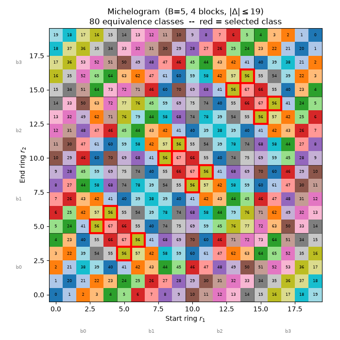
Michelogram coloured by equivalence class

The michelogram is a square grid where the cell at column r1 and row r2 represents sinogram plane (r1, r2). Cells that fall outside |r1 - r2| <= max_ring_diff are masked (shown in light grey).

Each colour corresponds to one equivalence class. Cells sharing a colour carry the same expected count for any cylindrically-symmetric object – only one of them needs to be computed. Thin black lines mark the boundaries between axial detector blocks.

The red outlines highlight all planes that belong to the same class as the selected plane (r1_sel, r2_sel). Their scatter across the michelogram illustrates how the three axial symmetries connect distant ring pairs.

Note

Cells are labelled with their class index. Cells of the same colour always share the same label, regardless of their position.

fig_mich, ax_mich = plt.subplots(figsize=(7, 7), tight_layout=True)
draw_michelogram(
    ax_mich,
    B,
    num_blocks,
    max_ring_diff,
    plane_to_class,
    class_to_planes,
    num_classes,
    highlight_pair=(r1_sel, r2_sel),
)
fig_mich.show()

Equivalent LORs for the selected plane

plane_orbit() returns all ring pairs in the same equivalence class as the seed pair (r1_sel, r2_sel). draw_panel renders these as lines between the two detector rows, using a small 8-sided scanner cross-section for illustration.

Crystals are coloured from dark (low sensitivity) to bright magenta (high sensitivity) according to their cosine-weighted axial sensitivity profile. Crystals in the outermost n_edge rings are shown in grey to indicate that they belong to the edge category and are therefore kept in separate classes.

Blue solid lines connect ring pairs with r2 > r1 (positive ring difference Delta); orange dashed lines show the swapped (r2, r1) pairs. All drawn lines are members of the same equivalence class and contribute equally to the geometric sensitivity of a symmetric object.

Note

The annotation box shows the intra-block crystal positions k = (r1 % B, r2 % B) together with the product of their sensitivity weights epsilon * epsilon. This product is the same for every plane in the class – it is the quantity that the block-shift symmetry preserves.

fig_panel, ax_panel = plt.subplots(figsize=(10, 5), tight_layout=True)
draw_panel(
    ax_panel,
    B,
    num_blocks,
    r1_sel,
    r2_sel,
    class_idx=cls_sel,
    n_edge=n_edge,
)
fig_panel.show()

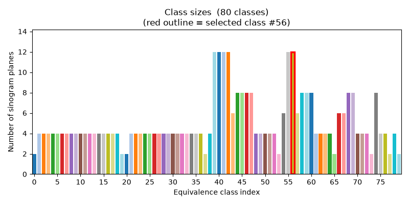
Class-size distribution

The bar chart shows how many sinogram planes belong to each equivalence class. Bars are coloured with the same palette as the michelogram, so each bar can be matched visually to its class.

For a scanner with num_blocks identical blocks and no edge correction all bars have equal height: each equivalence class contains exactly the same number of planes. When n_edge > 0 some classes become smaller because edge planes are grouped separately from interior planes.

Note

In practice the class-size distribution directly reveals the compression ratio of the symmetry reduction. If all classes have size m, a full sensitivity sinogram of N_planes planes can be replaced by N_planes / m unique computations, giving an exact m-fold speed-up for geometric sensitivity estimation.

fig_bar, ax_bar = plt.subplots(figsize=(8, 4), tight_layout=True)
draw_class_sizes(ax_bar, class_to_planes, num_classes, highlight_cls=cls_sel)
fig_bar.show()

In-plane symmetries

On top of the axial plane symmetries two more symmetries act on the view and radial-bin axes of the sinogram.

• build_view_class_indices() groups views by scanner rotational symmetry: views v, v + n, v + 2n, ... (where n = num_lor_endpoints_per_side) are all related by a rotation of the polygon scanner by one detector-block step. There are n distinct view classes, each containing num_views // n views.

• build_radial_class_indices() groups radial bins by the FOV mirror symmetry: bins r and num_rad - 1 - r carry the same perpendicular distance from the scanner axis and are therefore equivalent. Because num_rad is always odd for regular-polygon scanners there is a unique centre bin that forms a singleton class.

The combined reduction factor across all three axes is the product of the individual factors.

view_period = scanner.num_lor_endpoints_per_side
view_classes = build_view_class_indices(lor_desc.num_views, view_period)
rad_classes = build_radial_class_indices(lor_desc.num_rad)

n_view_classes = len(view_classes)
n_rad_classes = len(rad_classes)
views_per_class = lor_desc.num_views // n_view_classes
rads_per_class_max = max(len(c) for c in rad_classes)

reduction_planes = len(plane_to_class) / num_classes
reduction_views = lor_desc.num_views / n_view_classes
reduction_rad = lor_desc.num_rad / n_rad_classes
reduction_total = reduction_planes * reduction_views * reduction_rad

print(f"In-plane symmetries")
print(
    f"  View axis  : {lor_desc.num_views} views -> {n_view_classes} classes  "
    f"({views_per_class} views each,  "
    f"reduction factor {reduction_views:.1f}x)"
)
print(
    f"  Radial axis: {lor_desc.num_rad} bins  -> {n_rad_classes} classes  "
    f"(up to {rads_per_class_max} bins each,  "
    f"reduction factor {reduction_rad:.2f}x)"
)
print(f"Axial plane symmetry reduction factor : {reduction_planes:.1f}x")
print(
    f"Combined reduction (planes x views x radial) : "
    f"{reduction_total:.1f}x  "
    f"({len(plane_to_class) * lor_desc.num_views * lor_desc.num_rad} -> "
    f"{num_classes * n_view_classes * n_rad_classes} unique bins)"
)

In-plane symmetries
  View axis  : 224 views -> 16 classes  (14 views each,  reduction factor 14.0x)
  Radial axis: 441 bins  -> 221 classes  (up to 2 bins each,  reduction factor 2.00x)
Axial plane symmetry reduction factor : 5.0x
Combined reduction (planes x views x radial) : 139.7x  (39513600 -> 282880 unique bins)

Reducing a sinogram over equivalence classes

Given any sinogram (e.g. a Monte-Carlo emission scan of a uniform cylinder, or a forward-projection of a sensitivity phantom), the three index lists built above can be passed to reduce_sinogram_by_symmetry_class() to contract each axis down to its unique equivalence classes. The reductions are applied one axis at a time and can be chained in any order.

The reduce_sinogram_by_symmetry_class() function accepts an optional reduction argument:

Note

• reduction=xp.sum (default) – accumulates all counts within a class into a single bin. The total count across the whole sinogram is preserved. This is the right choice when reducing noisy Monte-Carlo data before dividing by a forward projection to obtain a per-class sensitivity estimate.

• reduction=xp.mean – normalises by class size, so every reduced bin holds the average count per original bin. Useful when you want the result to be directly comparable to a single unreduced bin value.

Here we demonstrate with a Poisson-noise sinogram drawn from a uniform expected value of 10 counts per bin. After reduction the shape shrinks from (num_rad, num_views, num_planes) to (n_rad_classes, n_view_classes, n_plane_classes), and the total count across all bins is exactly preserved.

np.random.seed(42)
sino = xp.asarray(
    np.random.poisson(10, lor_desc.spatial_sinogram_shape).astype(np.float64),
    device=dev,
)

# Build the per-class plane index arrays (requires a span-1 descriptor)
plane_class_idx = build_plane_class_indices(
    lor_desc.michelogram.plane_for_ring_pair_table, class_to_planes, num_classes
)

print(f"Sinogram shape before reduction : {tuple(sino.shape)}")

# Apply the three reductions in sequence: view -> radial -> plane
sino_red = reduce_sinogram_by_symmetry_class(
    sino, view_classes, lor_desc.view_axis_num, xp.sum
)
sino_red = reduce_sinogram_by_symmetry_class(
    sino_red, rad_classes, lor_desc.radial_axis_num, xp.sum
)
sino_red = reduce_sinogram_by_symmetry_class(
    sino_red, plane_class_idx, lor_desc.plane_axis_num, xp.sum
)

print(f"Sinogram shape after  reduction : {tuple(sino_red.shape)}")
print(f"Total counts before : {float(xp.sum(sino)):.0f}")
print(
    f"Total counts after  : {float(xp.sum(sino_red)):.0f}"
    f"  (preserved -- xp.sum reduction conserves total)"
)

Sinogram shape before reduction : (441, 224, 400)
Sinogram shape after  reduction : (221, 16, 80)
Total counts before : 395113764
Total counts after  : 395113764  (preserved -- xp.sum reduction conserves total)

Upsampling the reduced sinogram back to the original shape

After reducing with xp.mean every bin in the reduced sinogram holds the average count across all original bins that belong to the same equivalence class. expand_sinogram_by_symmetry_class() broadcasts those class values back to the original sinogram shape by assigning every original bin the mean value of its class. The result is a denoised sinogram in which symmetry-equivalent LORs carry identical values.

# -- Mean reduction ------------------------------------------------------------
sino_mean = reduce_sinogram_by_symmetry_class(
    sino, view_classes, lor_desc.view_axis_num, xp.mean
)
sino_mean = reduce_sinogram_by_symmetry_class(
    sino_mean, rad_classes, lor_desc.radial_axis_num, xp.mean
)
sino_mean = reduce_sinogram_by_symmetry_class(
    sino_mean, plane_class_idx, lor_desc.plane_axis_num, xp.mean
)
print(f"Reduced (mean) shape : {tuple(sino_mean.shape)}")

# -- Expand back to full sinogram shape ----------------------------------------
sino_expanded = expand_sinogram_by_symmetry_class(
    sino_mean, plane_class_idx, lor_desc.num_planes, lor_desc.plane_axis_num
)
sino_expanded = expand_sinogram_by_symmetry_class(
    sino_expanded, rad_classes, lor_desc.num_rad, lor_desc.radial_axis_num
)
sino_expanded = expand_sinogram_by_symmetry_class(
    sino_expanded, view_classes, lor_desc.num_views, lor_desc.view_axis_num
)
print(f"Expanded shape       : {tuple(sino_expanded.shape)}  (== original)")

# -- Verify: all bins in the same class carry the same value -------------------

sample_class_view = view_classes[3]  # e.g. class 3 of the view axis
sample_class_rad = rad_classes[0]  # outermost radial pair
sample_class_planes = xp.asarray(
    [lor_desc.michelogram.plane_for_ring_pair(*x) for x in class_to_planes[4]],
    device=dev,
)

r_idx, v_idx, p_idx = 0, 0, 0  # fix one radial and plane bin

vals_view = sino_expanded[r_idx, sample_class_view, p_idx]
print("")
print(f"View class 3 -- values at (rad={r_idx}, plane={p_idx})     : " f"{vals_view}")

vals_rad = sino_expanded[sample_class_rad, v_idx, p_idx]
print(f"Radial class 0   -- values at (view={v_idx}, plane={p_idx}): " f"{vals_rad}")


vals_planes = sino_expanded[r_idx, v_idx, sample_class_planes]

print(f"Plane class 4  -- values at (rad={r_idx}, view={v_idx})    : " f"{vals_planes}")

Reduced (mean) shape : (221, 16, 80)
Expanded shape       : (441, 224, 400)  (== original)

View class 3 -- values at (rad=0, plane=0)     : tensor([9.9821, 9.9821, 9.9821, 9.9821, 9.9821, 9.9821, 9.9821, 9.9821, 9.9821,
        9.9821, 9.9821, 9.9821, 9.9821, 9.9821], dtype=torch.float64)
Radial class 0   -- values at (view=0, plane=0): tensor([10.3214, 10.3214], dtype=torch.float64)
Plane class 4  -- values at (rad=0, view=0)    : tensor([10.0714, 10.0714, 10.0714, 10.0714], dtype=torch.float64)