LOR descriptors and sinogram definition

In a scanner with “cylindrical symmetry”, all possible lines of response (LORs) between two LOR endpoints can be sorted into a sinogram containing a radial, view and plane dimension. This example shows how this can be done using the RegularPolygonPETLORDescriptor

import numpy as np
import parallelproj.pet_scanners
import parallelproj.pet_lors
import matplotlib.pyplot as plt

from parallelproj._examples_utils import suggest_array_backend_and_device

# To use a specific backend and/or device, replace the None arguments, e.g.:
#   xp, dev = suggest_array_backend_and_device(backend="numpy", dev="cpu") or by setting xp and dev manually
xp, dev = suggest_array_backend_and_device(None, None)

Using array API: array_api_compat.torch, device: cpu

def _central_plane_seg0(
    lor_desc: parallelproj.pet_lors.RegularPolygonPETLORDescriptor,
) -> int:
    """Return the plane index of the central plane belonging to segment 0."""
    seg = np.asarray(lor_desc.plane_segment.tolist())
    idx = np.where(seg == 0)[0]
    return int(idx[len(idx) // 2])


def _last_plane_highest_seg(
    lor_desc: parallelproj.pet_lors.RegularPolygonPETLORDescriptor,
) -> int:
    """Return the last plane index belonging to the highest-magnitude segment."""
    seg = np.asarray(lor_desc.plane_segment.tolist())
    idx = np.where(np.abs(seg) == int(np.abs(seg).max()))[0]
    return int(idx[-1])

setup a small regular polygon PET scanner with 11 rings (polygons)

num_rings = 11
scanner = parallelproj.pet_scanners.RegularPolygonPETScannerGeometry(
    xp,
    dev,
    radius=65.0,
    num_sides=12,
    num_lor_endpoints_per_side=4,
    lor_spacing=8.0,
    ring_positions=2 * num_rings * xp.linspace(-1, 1, num_rings, device=dev),
    symmetry_axis=2,
)

Defining a sinogram using an LOR descriptor

RegularPolygonPETLORDescriptor can be used to order all possible combinations of LOR endpoints into a sinogram with a radial, view and plane dimension.

The maximum ring difference (passed via a Michelogram) defines which ring pairs form valid LORs, and radial_trim defines the number of radial bins to be trimmed from the sinogram edges.

sinogram_order of type SinogramSpatialAxisOrder defines the order of the sinogram dimensions (e.g. RVP -> [radial, view, plane], PRV -> [plane, radial, view])

lor_desc1 = parallelproj.pet_lors.RegularPolygonPETLORDescriptor(
    scanner,
    radial_trim=10,
    sinogram_order=parallelproj.pet_lors.SinogramSpatialAxisOrder.RVP,
)

print(lor_desc1)
print(f"sinogram order: {lor_desc1.sinogram_order.name}")
print(f"sinogram shape: {lor_desc1.spatial_sinogram_shape}")
print(
    f"num rad: {lor_desc1.num_rad}  num views: {lor_desc1.num_views}  num planes: {lor_desc1.num_planes}"
)
print(
    f"radial axis num: {lor_desc1.radial_axis_num}  view axis num: {lor_desc1.view_axis_num}  plane axis num: {lor_desc1.plane_axis_num}"
)

RegularPolygonPETLORDescriptor with spatial sinogram shape (27R, 24V, 121P)
sinogram order: RVP
sinogram shape: (27, 24, 121)
num rad: 27  num views: 24  num planes: 121
radial axis num: 0  view axis num: 1  plane axis num: 2

Define a 2nd LOR descriptor with sinogram order “PRV”

lor_desc2 = parallelproj.pet_lors.RegularPolygonPETLORDescriptor(
    scanner,
    radial_trim=10,
    sinogram_order=parallelproj.pet_lors.SinogramSpatialAxisOrder.PRV,
)

print(lor_desc2)
print(f"sinogram order: {lor_desc2.sinogram_order.name}")
print(f"sinogram shape: {lor_desc2.spatial_sinogram_shape}")
print(
    f"num rad: {lor_desc2.num_rad}  num views: {lor_desc2.num_views}  num planes: {lor_desc2.num_planes}"
)
print(
    f"radial axis num: {lor_desc2.radial_axis_num}  view axis num: {lor_desc2.view_axis_num}  plane axis num: {lor_desc2.plane_axis_num}"
)

RegularPolygonPETLORDescriptor with spatial sinogram shape (121P, 27R, 24V)
sinogram order: PRV
sinogram shape: (121, 27, 24)
num rad: 27  num views: 24  num planes: 121
radial axis num: 1  view axis num: 2  plane axis num: 0

Obtaining world coordinates of LOR start and endpoints

Every LOR is defined by two LOR endpoints. RegularPolygonPETLORDescriptor.get_lor_coordinates() can be used to to obtain the 3 world coordinates of them (for all views or a subset of views).

lor_start_points1, lor_end_points1 = lor_desc1.get_lor_coordinates()
print(lor_start_points1.shape, lor_end_points1.shape)

# print the start and end coordinates of the LOR corresponding to the 1st view
# the 2nd plane and the 3rd radial bin
print(lor_start_points1[2, 0, 1, :])
print(lor_end_points1[2, 0, 1, :])

torch.Size([27, 24, 121, 3]) torch.Size([27, 24, 121, 3])
tensor([-54.2916, -35.9641, -17.6000])
tensor([-29.0359,  58.2916, -17.6000])

Do the same for the 2nd LOR descriptor that uses sinogram order “PRV” The indexing has to be different compared to “RVP” to get the same LOR.

lor_start_points2, lor_end_points2 = lor_desc2.get_lor_coordinates()
print(lor_start_points2.shape, lor_end_points2.shape)

# print the start and end coordinates of the LOR corresponding to the 1st view
# the 2nd plane and the 3rd radial bin
print(lor_start_points2[1, 2, 0, :])
print(lor_end_points2[1, 2, 0, :])

torch.Size([121, 27, 24, 3]) torch.Size([121, 27, 24, 3])
tensor([-54.2916, -35.9641, -17.6000])
tensor([-29.0359,  58.2916, -17.6000])

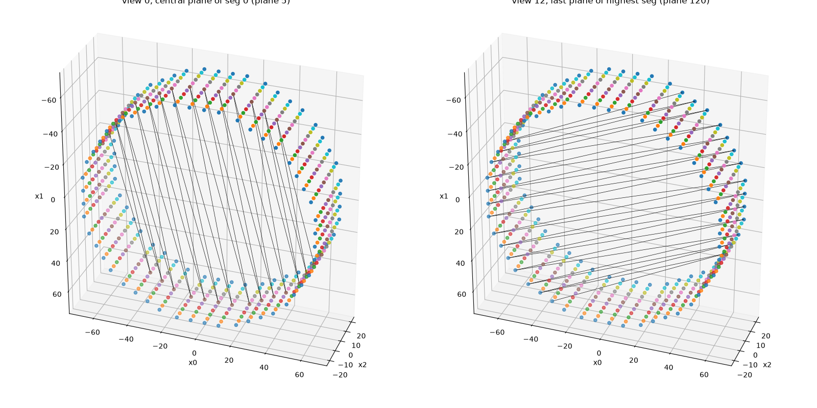
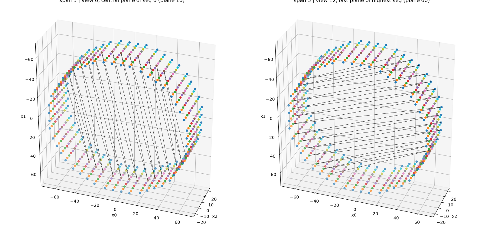
Visualize the defined LOR endpoints

RegularPolygonPETScannerGeometry.show_lor_endpoints() can be used to visualize the defined LOR endpoints. Note that a zig-zag sampling pattern is used to define a view.

_p0 = _central_plane_seg0(lor_desc1)
_ph = _last_plane_highest_seg(lor_desc1)

fig = plt.figure(figsize=(16, 8), tight_layout=True)
ax1 = fig.add_subplot(121, projection="3d")
ax2 = fig.add_subplot(122, projection="3d")
for ax in (ax1, ax2):
    ax.view_init(elev=-30, azim=160, roll=180, vertical_axis="y")
scanner.show_lor_endpoints(ax1)
lor_desc1.show_views(
    ax1,
    views=xp.asarray([0], device=dev),
    planes=xp.asarray([_p0], device=dev),
    lw=0.5,
    color="k",
)
ax1.set_title(f"view 0, central plane of seg 0 (plane {_p0})")
scanner.show_lor_endpoints(ax2)
lor_desc1.show_views(
    ax2,
    views=xp.asarray([lor_desc1.num_views // 2], device=dev),
    planes=xp.asarray([_ph], device=dev),
    lw=0.5,
    color="k",
)
ax2.set_title(
    f"view {lor_desc1.num_views // 2}, last plane of highest seg (plane {_ph})"
)
fig.show()

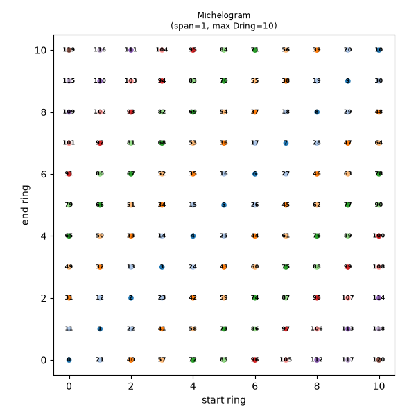
Michelogram for span-1 (no max ring diff)

fig_m0, ax_m0 = plt.subplots(1, 1, figsize=(6, 6), tight_layout=True)
lor_desc1.show_michelogram(ax_m0)
fig_m0.show()

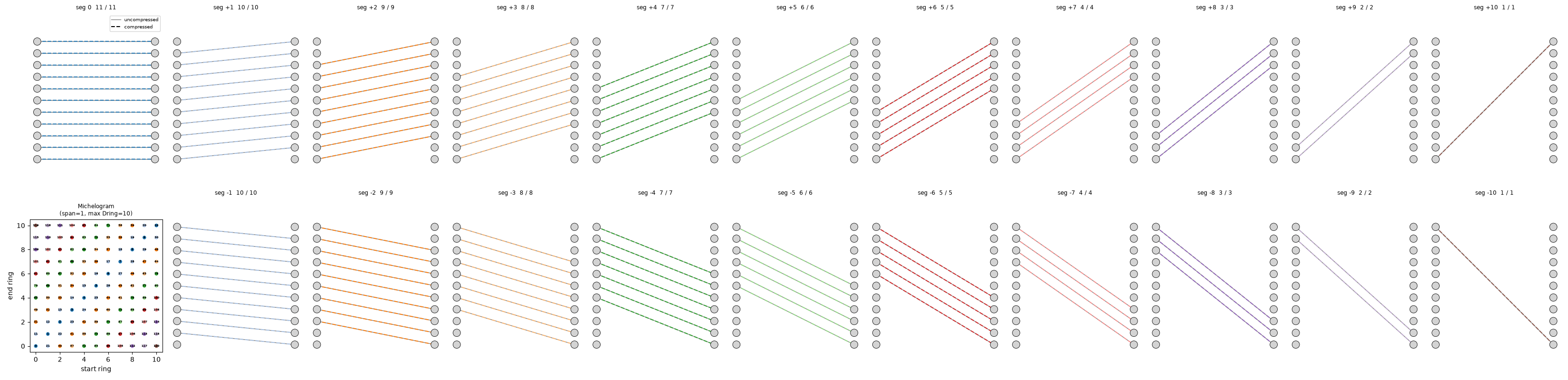
Segment side-view diagram for span-1 (no max ring diff)

fig_seg0 = lor_desc1.show_segment_lors()
fig_seg0.tight_layout()
fig_seg0.show()

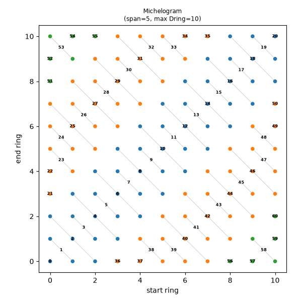
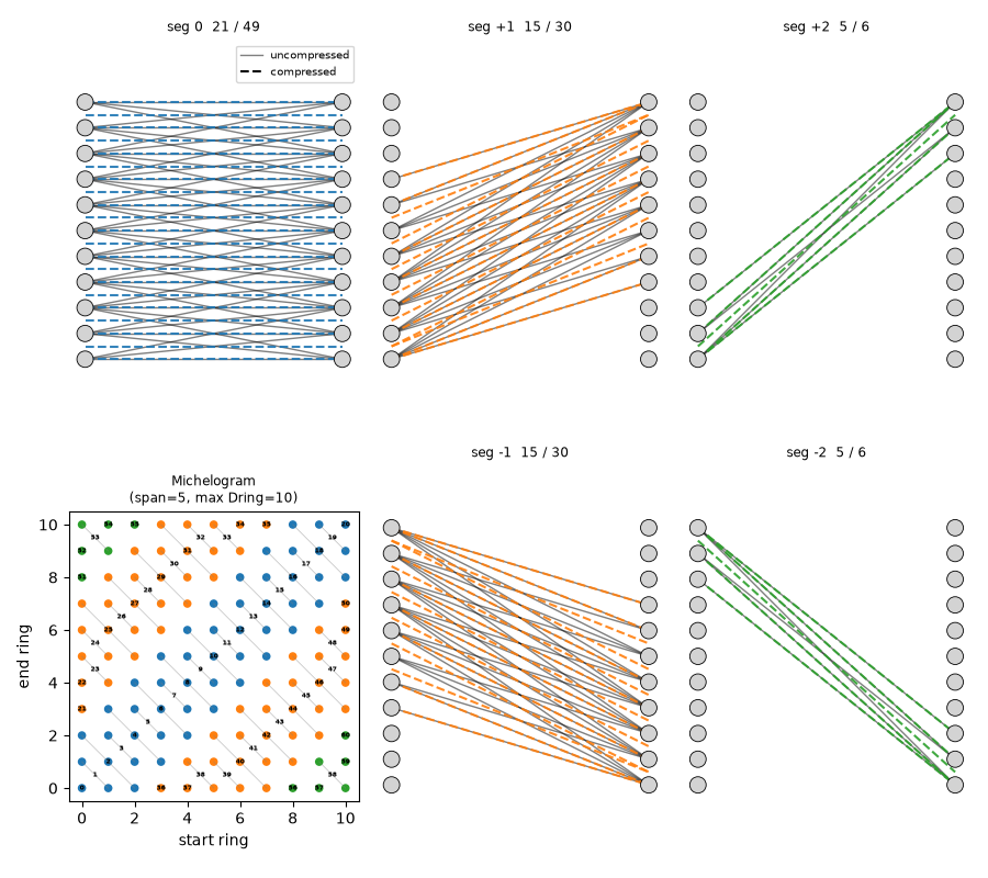
Span-5 sinogram without max ring difference limitation

RegularPolygonPETLORDescriptor supports axial compression via the span parameter. With span=5 ring pairs whose ring difference falls in the same segment and share the same axial midpoint are merged into a single sinogram plane. Passing max_ring_difference=scanner.num_rings - 1 to the Michelogram includes all ring pairs.

span = 5

lor_desc_s5 = parallelproj.pet_lors.RegularPolygonPETLORDescriptor(
    scanner,
    parallelproj.pet_lors.Michelogram(
        scanner.num_rings, max_ring_difference=scanner.num_rings - 1, span=span
    ),
    radial_trim=10,
    sinogram_order=parallelproj.pet_lors.SinogramSpatialAxisOrder.RVP,
)

print(lor_desc_s5)
print(f"sinogram shape: {lor_desc_s5.spatial_sinogram_shape}")
print(f"num planes: {lor_desc_s5.num_planes}  (span={span}, no max ring diff)")

RegularPolygonPETLORDescriptor with spatial sinogram shape (27R, 24V, 61P)
sinogram shape: (27, 24, 61)
num planes: 61  (span=5, no max ring diff)

Michelogram for span-5 (no max ring diff)

fig_m1, ax_m1 = plt.subplots(1, 1, figsize=(6, 6), tight_layout=True)
lor_desc_s5.show_michelogram(ax_m1)
fig_m1.show()

Segment side-view diagram for span-5 (no max ring diff)

fig_seg1 = lor_desc_s5.show_segment_lors()
fig_seg1.tight_layout()
fig_seg1.show()

3D visualisation of two planes - span-5 (no max ring diff)

_p0_s5 = _central_plane_seg0(lor_desc_s5)
_ph_s5 = _last_plane_highest_seg(lor_desc_s5)

fig_3d1 = plt.figure(figsize=(16, 8), tight_layout=True)
ax3d1a = fig_3d1.add_subplot(121, projection="3d")
ax3d1b = fig_3d1.add_subplot(122, projection="3d")
for ax in (ax3d1a, ax3d1b):
    ax.view_init(elev=-30, azim=160, roll=180, vertical_axis="y")
scanner.show_lor_endpoints(ax3d1a)
lor_desc_s5.show_views(
    ax3d1a,
    views=xp.asarray([0], device=dev),
    planes=xp.asarray([_p0_s5], device=dev),
    lw=0.5,
    color="k",
)
ax3d1a.set_title(f"span {span} | view 0, central plane of seg 0 (plane {_p0_s5})")
scanner.show_lor_endpoints(ax3d1b)
lor_desc_s5.show_views(
    ax3d1b,
    views=xp.asarray([lor_desc_s5.num_views // 2], device=dev),
    planes=xp.asarray([_ph_s5], device=dev),
    lw=0.5,
    color="k",
)
ax3d1b.set_title(
    f"span {span} | view {lor_desc_s5.num_views // 2}, last plane of highest seg (plane {_ph_s5})"
)
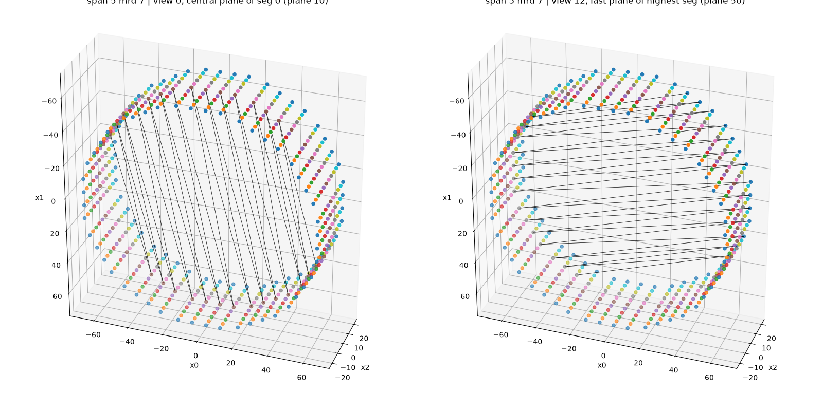
fig_3d1.show()

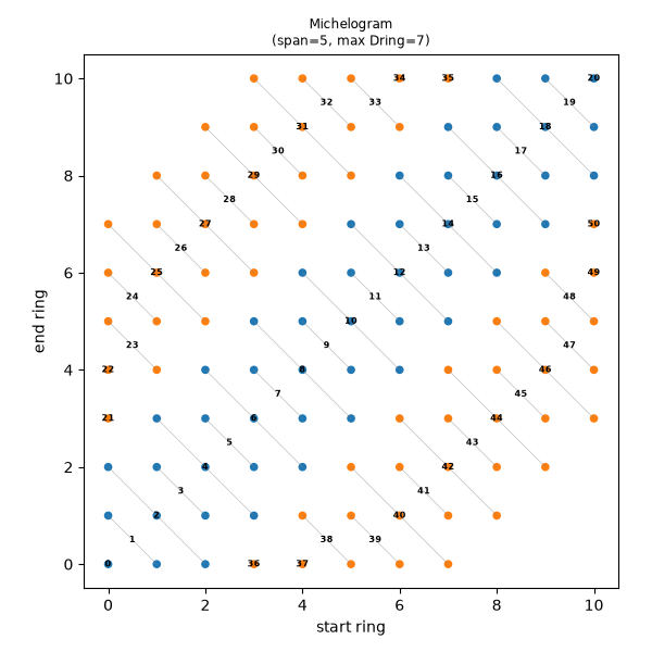
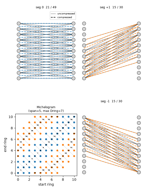
Span-5 sinogram with max ring difference = 7

By additionally setting max_ring_difference=7 we restrict the included ring pairs, reducing the number of segments and sinogram planes compared to the unrestricted span-5 case above.

max_ring_difference = 7

lor_desc_s5_mrd9 = parallelproj.pet_lors.RegularPolygonPETLORDescriptor(
    scanner,
    parallelproj.pet_lors.Michelogram(
        scanner.num_rings, max_ring_difference=max_ring_difference, span=span
    ),
    radial_trim=10,
    sinogram_order=parallelproj.pet_lors.SinogramSpatialAxisOrder.RVP,
)

print(lor_desc_s5_mrd9)
print(f"sinogram shape: {lor_desc_s5_mrd9.spatial_sinogram_shape}")
print(
    f"num planes: {lor_desc_s5_mrd9.num_planes}  (span={span}, max ring diff={max_ring_difference})"
)

RegularPolygonPETLORDescriptor with spatial sinogram shape (27R, 24V, 51P)
sinogram shape: (27, 24, 51)
num planes: 51  (span=5, max ring diff=7)

Michelogram for span-5 with max ring diff = 7

fig_m2, ax_m2 = plt.subplots(1, 1, figsize=(6, 6), tight_layout=True)
lor_desc_s5_mrd9.show_michelogram(ax_m2)
fig_m2.show()

Segment side-view diagram for span-5 with max ring diff = 7

fig_seg2 = lor_desc_s5_mrd9.show_segment_lors()
fig_seg2.tight_layout()
fig_seg2.show()

3D visualisation of two planes - span-5, max ring diff = 7

_p0_s5_mrd9 = _central_plane_seg0(lor_desc_s5_mrd9)
_ph_s5_mrd9 = _last_plane_highest_seg(lor_desc_s5_mrd9)

fig_3d2 = plt.figure(figsize=(16, 8), tight_layout=True)
ax3d2a = fig_3d2.add_subplot(121, projection="3d")
ax3d2b = fig_3d2.add_subplot(122, projection="3d")
for ax in (ax3d2a, ax3d2b):
    ax.view_init(elev=-30, azim=160, roll=180, vertical_axis="y")
scanner.show_lor_endpoints(ax3d2a)
lor_desc_s5_mrd9.show_views(
    ax3d2a,
    views=xp.asarray([0], device=dev),
    planes=xp.asarray([_p0_s5_mrd9], device=dev),
    lw=0.5,
    color="k",
)
ax3d2a.set_title(
    f"span {span} mrd {max_ring_difference} | view 0, central plane of seg 0 (plane {_p0_s5_mrd9})"
)
scanner.show_lor_endpoints(ax3d2b)
lor_desc_s5_mrd9.show_views(
    ax3d2b,
    views=xp.asarray([lor_desc_s5_mrd9.num_views // 2], device=dev),
    planes=xp.asarray([_ph_s5_mrd9], device=dev),
    lw=0.5,
    color="k",
)
ax3d2b.set_title(
    f"span {span} mrd {max_ring_difference} | view {lor_desc_s5_mrd9.num_views // 2}, last plane of highest seg (plane {_ph_s5_mrd9})"
)
fig_3d2.show()

GE-style plane ordering

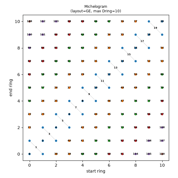
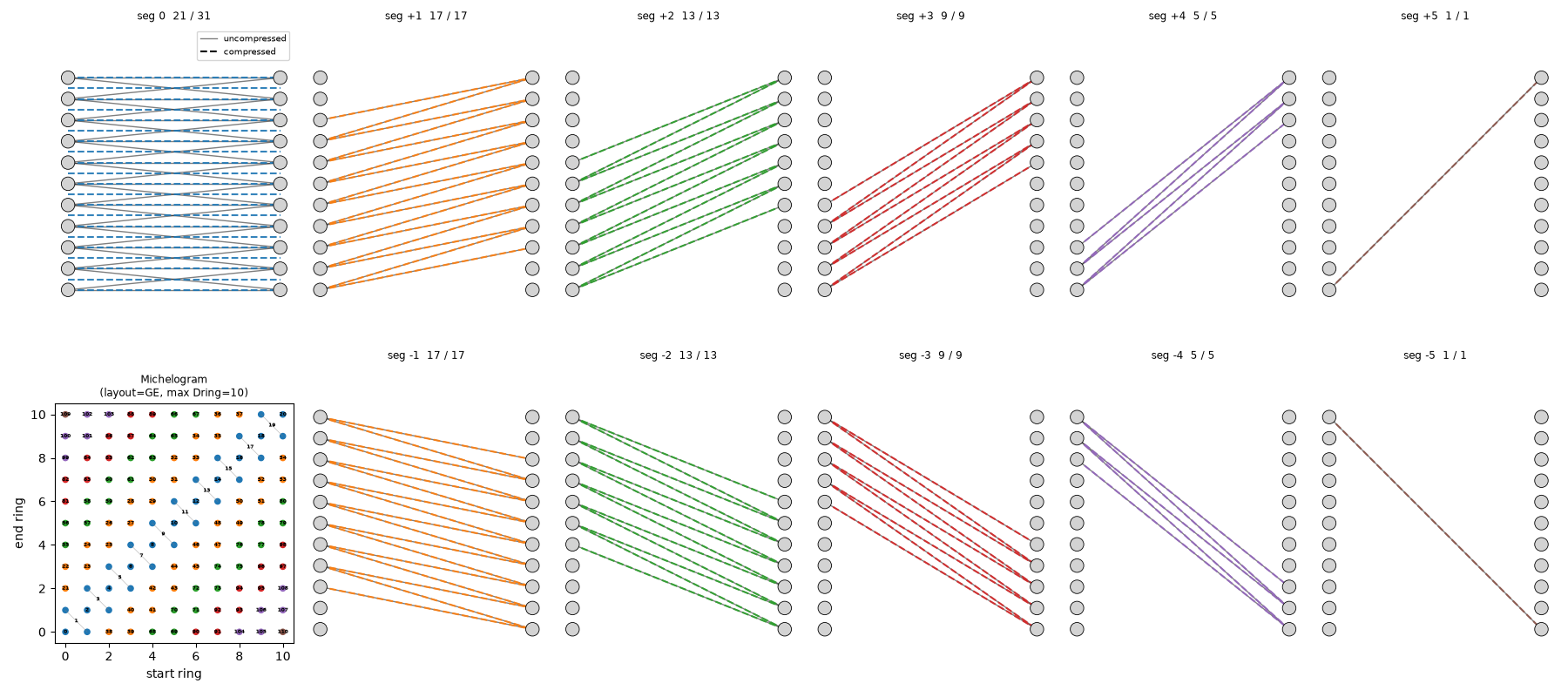
Instead of a single (odd) span, GE-style scanners use a mixed axial layout: segment 0 collects ring differences {-1, 0, +1} (the +/-1 cross planes are merged into virtual direct planes), while every oblique segment collects a ring-difference pair {+/-2k, +/-(2k+1)} laid out as a staircase. Select it with the Michelogram.ge() constructor (equivalently layout=MichelogramLayout.GE); span is then ignored and Michelogram.span returns None. Choose num_rings and max_ring_difference to match the GE scanner of interest.

lor_desc_ge = parallelproj.pet_lors.RegularPolygonPETLORDescriptor(
    scanner,
    parallelproj.pet_lors.Michelogram.ge(
        scanner.num_rings, max_ring_difference=scanner.num_rings - 1
    ),
    radial_trim=10,
    sinogram_order=parallelproj.pet_lors.SinogramSpatialAxisOrder.RVP,
)

print(lor_desc_ge)
print(f"sinogram shape: {lor_desc_ge.spatial_sinogram_shape}")
print(f"num planes: {lor_desc_ge.num_planes}  (GE layout, span={lor_desc_ge.span})")

RegularPolygonPETLORDescriptor with spatial sinogram shape (27R, 24V, 111P)
sinogram shape: (27, 24, 111)
num planes: 111  (GE layout, span=None)

Michelogram for the GE-style layout

fig_mge, ax_mge = plt.subplots(1, 1, figsize=(6, 6), tight_layout=True)
lor_desc_ge.show_michelogram(ax_mge)
fig_mge.show()

Segment side-view diagram for the GE-style layout

fig_seg_ge = lor_desc_ge.show_segment_lors()
fig_seg_ge.tight_layout()
fig_seg_ge.show()

Sinogram indexing conventions (all the knobs)

The mapping between a sinogram bin (view, radial) and the underlying pair of detectors is fixed by a small set of orthogonal knobs. By default, view 0’s central radial bin connects detector 0 and detector N/2 (diametrically opposing). The knobs then let you reproduce any vendor’s convention:

• ring_endpoint_ordering (on the scanner) – physical crystal numbering direction around the ring (CLOCKWISE / COUNTERCLOCKWISE).

• phi0 (on the scanner) – azimuth of module 0. The default 0 places module 0 on the -y axis (top of the default view) for symmetry_axis=2.

• zig_zag_order – which endpoint takes the interleaving half-step (END_FIRST / START_FIRST).

• view_direction – direction in which the view index advances (PLUS / MINUS).

• radial_direction – direction in which the radial index advances.

view_direction / radial_direction flip the sinogram bin layout while ring_endpoint_ordering flips the physical crystal numbering – three independent choices that together span every regular-polygon convention.

pl = parallelproj.pet_lors

# A *minimal* 1-ring scanner (4 sides x 2 endpoints = 8 detectors) so the full
# detector <-> (view, radial) tables fit on screen.
mini = parallelproj.pet_scanners.RegularPolygonPETScannerGeometry(
    xp,
    dev,
    radius=30.0,
    num_sides=4,
    num_lor_endpoints_per_side=2,
    lor_spacing=12.0,
    ring_positions=xp.asarray([0.0], device=dev),
    symmetry_axis=2,
)
Nmini = mini.num_lor_endpoints_per_ring  # = 8


def _print_table(d: pl.RegularPolygonPETLORDescriptor, title: str) -> None:
    """Print the full (view, radial) -> ``start-end`` detector-index table."""
    s = np.asarray(parallelproj.to_numpy_array(d.start_in_ring_index))
    e = np.asarray(parallelproj.to_numpy_array(d.end_in_ring_index))
    print(f"\n{title}   (view 0 central bin -> detectors (0, {Nmini // 2}))")
    print("  radial bin :", " ".join(f"{r:>3d}" for r in range(d.num_rad)))
    for v in range(d.num_views):
        row = " ".join(f"{int(s[v, r])}-{int(e[v, r])}" for r in range(d.num_rad))
        print(f"  view {v}     :", row)


d0 = pl.RegularPolygonPETLORDescriptor(mini, radial_trim=0)
_print_table(d0, "default")
_print_table(
    pl.RegularPolygonPETLORDescriptor(
        mini, radial_trim=0, view_direction=pl.ViewDirection.MINUS
    ),
    "view_direction=MINUS",
)
_print_table(
    pl.RegularPolygonPETLORDescriptor(
        mini, radial_trim=0, radial_direction=pl.RadialDirection.MINUS
    ),
    "radial_direction=MINUS",
)
_print_table(
    pl.RegularPolygonPETLORDescriptor(
        mini, radial_trim=0, zig_zag_order=pl.SinogramZigZagOrder.START_FIRST
    ),
    "zig_zag_order=START_FIRST",
)

# ``ring_endpoint_ordering`` is a *scanner* knob: it changes the physical
# crystal numbering (mirrors detector positions) but not the (view, radial)
# index formula, so the table above is unchanged while detector 1 moves.
mini_ccw = parallelproj.pet_scanners.RegularPolygonPETScannerGeometry(
    xp,
    dev,
    radius=30.0,
    num_sides=4,
    num_lor_endpoints_per_side=2,
    lor_spacing=12.0,
    ring_positions=xp.asarray([0.0], device=dev),
    symmetry_axis=2,
    ring_endpoint_ordering=parallelproj.pet_scanners.RingEndpointOrdering.COUNTERCLOCKWISE,
)
_ep_cw = np.asarray(parallelproj.to_numpy_array(mini.all_lor_endpoints)).reshape(-1, 3)
_ep_ccw = np.asarray(parallelproj.to_numpy_array(mini_ccw.all_lor_endpoints)).reshape(
    -1, 3
)
print(
    "\ndetector 1 position (x, y):  CW =",
    np.round(_ep_cw[1, :2], 1),
    "  CCW =",
    np.round(_ep_ccw[1, :2], 1),
)

default   (view 0 central bin -> detectors (0, 4))
  radial bin :   0   1   2   3   4   5   6
  view 0     : 6-5 7-5 7-4 0-4 0-3 1-3 1-2
  view 1     : 7-6 0-6 0-5 1-5 1-4 2-4 2-3
  view 2     : 0-7 1-7 1-6 2-6 2-5 3-5 3-4
  view 3     : 1-0 2-0 2-7 3-7 3-6 4-6 4-5

view_direction=MINUS   (view 0 central bin -> detectors (0, 4))
  radial bin :   0   1   2   3   4   5   6
  view 0     : 6-5 7-5 7-4 0-4 0-3 1-3 1-2
  view 1     : 5-4 6-4 6-3 7-3 7-2 0-2 0-1
  view 2     : 4-3 5-3 5-2 6-2 6-1 7-1 7-0
  view 3     : 3-2 4-2 4-1 5-1 5-0 6-0 6-7

radial_direction=MINUS   (view 0 central bin -> detectors (0, 4))
  radial bin :   0   1   2   3   4   5   6
  view 0     : 1-2 1-3 0-3 0-4 7-4 7-5 6-5
  view 1     : 2-3 2-4 1-4 1-5 0-5 0-6 7-6
  view 2     : 3-4 3-5 2-5 2-6 1-6 1-7 0-7
  view 3     : 4-5 4-6 3-6 3-7 2-7 2-0 1-0

zig_zag_order=START_FIRST   (view 0 central bin -> detectors (0, 4))
  radial bin :   0   1   2   3   4   5   6
  view 0     : 7-6 7-5 0-5 0-4 1-4 1-3 2-3
  view 1     : 0-7 0-6 1-6 1-5 2-5 2-4 3-4
  view 2     : 1-0 1-7 2-7 2-6 3-6 3-5 4-5
  view 3     : 2-1 2-0 3-0 3-7 4-7 4-6 5-6

detector 1 position (x, y):  CW = [  6. -30.]   CCW = [ -6. -30.]

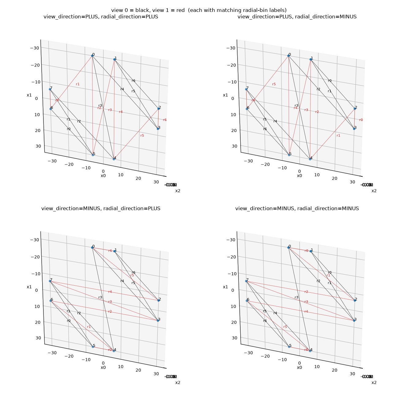
Visualise the four (ViewDirection, RadialDirection) combinations

2x2 panel of the minimal scanner. Detector numbers are annotated; view 0 is drawn in black and view 1 in red, each with its own radial-bin labels (in the matching line colour), so the effect of view_direction (which way the views advance) is visible. View 0’s central bin always connects detector 0 and detector N/2.

def _draw_panel(ax, view_direction, radial_direction):
    ax.view_init(elev=-30, azim=160, roll=180, vertical_axis="y")  # look down the ring (z) axis
    mini.show_lor_endpoints(ax, annotation_fontsize=9, show_linear_index=True)
    d = pl.RegularPolygonPETLORDescriptor(
        mini,
        radial_trim=0,
        view_direction=view_direction,
        radial_direction=radial_direction,
    )
    xs, xe = d.get_lor_coordinates(views=xp.asarray([0, 1], device=dev))
    xs = np.asarray(parallelproj.to_numpy_array(xs))
    xe = np.asarray(parallelproj.to_numpy_array(xe))
    ra, va, pa = d.radial_axis_num, d.view_axis_num, d.plane_axis_num
    # LOR colour per view; the radial-bin labels use the matching line colour
    for vi, col, lab_col in ((0, "k", "k"), (1, "tab:red", "tab:red")):
        for r in range(d.num_rad):
            idx = [0, 0, 0]
            idx[ra], idx[va], idx[pa] = r, vi, 0
            a, b = xs[tuple(idx)], xe[tuple(idx)]
            ax.plot([a[0], b[0]], [a[1], b[1]], [a[2], b[2]], color=col, lw=0.5)
            # nudge the two views' labels apart so the central bins don't overlap
            m = 0.5 * (a + b) + (2.0 if vi == 1 else -2.0)
            ax.text(m[0], m[1], m[2], f"r{r}", color=lab_col, fontsize=8)
    ax.set_title(
        f"view_direction={view_direction.name}, radial_direction={radial_direction.name}"
    )


fig_k = plt.figure(figsize=(13, 13), tight_layout=True)
_combos = [
    (pl.ViewDirection.PLUS, pl.RadialDirection.PLUS),
    (pl.ViewDirection.PLUS, pl.RadialDirection.MINUS),
    (pl.ViewDirection.MINUS, pl.RadialDirection.PLUS),
    (pl.ViewDirection.MINUS, pl.RadialDirection.MINUS),
]
for _i, (_vd, _rd) in enumerate(_combos):
    _draw_panel(fig_k.add_subplot(2, 2, _i + 1, projection="3d"), _vd, _rd)
fig_k.suptitle("view 0 = black, view 1 = red  (each with matching radial-bin labels)")
fig_k.show()

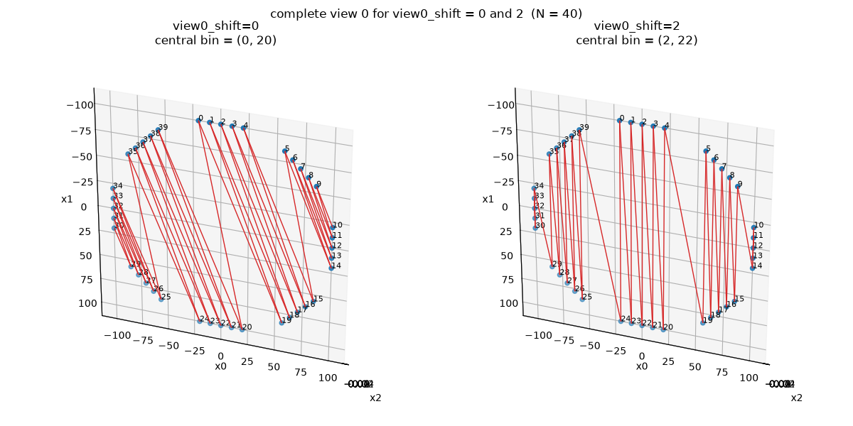
User-defined view-0 anchor shift (view0_shift)

By default view 0’s central radial bin connects detectors (0, N/2). The view0_shift=m argument (a non-negative integer) rotates the detector anchor of every view by m crystals, so view 0’s central bin instead connects ((0+m) mod N, (N/2+m) mod N). Below we draw the complete view 0 (all radial bins, via show_views()) on an 8-module x 5-crystal ring for m=0 (default) and m=2: the whole parallel set of LORs rotates by m crystals while the rest of the sinogram indexing is unchanged.

mini_shift = parallelproj.pet_scanners.RegularPolygonPETScannerGeometry(
    xp,
    dev,
    radius=100.0,
    num_sides=8,
    num_lor_endpoints_per_side=5,
    lor_spacing=10.0,
    ring_positions=xp.asarray([0.0], device=dev),
    symmetry_axis=2,
)

fig_sh, ax_sh = plt.subplots(
    1, 2, figsize=(12, 6), subplot_kw={"projection": "3d"}, tight_layout=True
)
for _ax, _m in zip(ax_sh, (0, 2)):
    _ax.view_init(elev=-30, azim=160, roll=180, vertical_axis="y")
    mini_shift.show_lor_endpoints(_ax, annotation_fontsize=8, show_linear_index=True)
    d = pl.RegularPolygonPETLORDescriptor(mini_shift, radial_trim=0, view0_shift=_m)
    d.show_views(
        _ax,
        views=xp.asarray([0], device=dev),
        planes=xp.asarray([0], device=dev),
        lw=1.0,
        color="tab:red",
    )
    s_idx = int(parallelproj.to_numpy_array(d.start_in_ring_index)[0, (d.num_rad - 1) // 2])
    e_idx = int(parallelproj.to_numpy_array(d.end_in_ring_index)[0, (d.num_rad - 1) // 2])
    _ax.set_title(f"view0_shift={_m}\ncentral bin = ({s_idx}, {e_idx})")
fig_sh.suptitle(
    f"complete view 0 for view0_shift = 0 and 2  "
    f"(N = {mini_shift.num_lor_endpoints_per_ring})"
)
fig_sh.show()

Typical vendor settings

The default is that view 0’s central bin connects detectors (0, N/2) and module 0 sits on -y (top of the default view). To line a descriptor up with a specific vendor’s sinograms you set a few knobs – there is no single “vendor” setting, because e.g. different vendors use opposite handedness:

• phi0 (scanner) – rotate module 0 to the vendor’s physical crystal-0 azimuth.

• ring_endpoint_ordering – match the vendor’s crystal numbering direction.

• view_direction / radial_direction – match the vendor’s sinogram bin ordering (vendors differ here).

• zig_zag_order – match the interleaving of adjacent LOR angles.

Rather than trusting a preset, verify the combination on your data. e.g. by backprojecting a sparse sinogram.